AMATH 251: Introduction to Differential Equations
Sue Ann Campbell
Estimated study time: 1 hr 19 min
Table of contents
Sources and References
Primary textbook — Edwards, Penney & Calvis, Differential Equations and Boundary Value Problems: Computing and Modeling, 5th ed. Supplementary texts —
- Boyce, DiPrima & Meade, Elementary Differential Equations and Boundary Value Problems, 11th ed.
- Strogatz, Nonlinear Dynamics and Chaos, 2nd ed.
- Tenenbaum & Pollard, Ordinary Differential Equations (Dover)
- Coddington & Levinson, Theory of Ordinary Differential Equations
- Lamb, Dimensional Analysis (lecture notes)
Online resources —
- MIT OpenCourseWare 18.03 Differential Equations — Mattuck/Miller lecture notes
- Paul’s Online Math Notes (Lamar University) — Laplace transform tables
- Khan Academy — slope field visualizations
Chapter 1: What Is a Differential Equation?
1.1 Modeling with Rates of Change
The simplest scientific observation about the world is that things change. A population grows, a capacitor discharges, a pendulum swings, a rumour spreads. What makes these phenomena mathematical is that the rate of change of a quantity often depends in a definite way on the quantity itself. A differential equation captures exactly this: a relationship between a function and its derivatives.
More formally, a differential equation (DE) is an equation that contains one or more derivatives of an unknown function. The function we are trying to find is the dependent variable and it depends on one or more independent variables. If there is only one independent variable the equation is an ordinary differential equation (ODE); if there are several, it is a partial differential equation (PDE). This course studies ODEs exclusively.
The standard example that motivated the subject is Newton’s second law: \(F = ma\). In the setting of a spring–mass system, \(F\) depends on position \(x\) and \(a = x''\), so Newton’s law instantly becomes an ODE. The same structure appears in circuit analysis (Kirchhoff’s voltage law gives a second-order ODE for charge), population biology (the logistic equation), thermodynamics (Newton’s law of cooling), and celestial mechanics. ODEs are, in Strogatz’s phrase, the language in which the laws of nature are written.
1.2 Order, Linearity, and Solutions
A second-order ODE looks like \(F(x, y, y', y'') = 0\) for some function \(F\). The unknown function \(y\) depends on the independent variable \(x\) (or \(t\) for time).
The distinction matters enormously for what solution methods are available. For linear equations we have the whole machinery of superposition: sums and scalar multiples of solutions are again solutions (in the homogeneous case), which lets us build up a general solution from a basis of particular ones. Nonlinear ODEs, by contrast, resist such structure and are far harder in general.
A general solution contains \(n\) arbitrary constants (one for each integration needed to drop from order \(n\) to order 0); a particular solution is one in which the constants have been fixed, typically by initial or boundary conditions.
1.3 Initial Value Problems and the Three Fundamental Questions
\[y^{(n)} = f(x, y, y', \ldots, y^{(n-1)}), \quad y(x_0)=y_0,\; y'(x_0)=y_1,\;\ldots\;,\; y^{(n-1)}(x_0)=y_{n-1}.\]Before trying to solve any IVP, three questions should be asked:
- Existence. Does a solution exist?
- Uniqueness. Is there only one solution satisfying the given conditions?
- Dependence on data. How sensitively does the solution change when the initial conditions or parameters are perturbed?
The first two questions are answered for first-order equations by the following fundamental result.
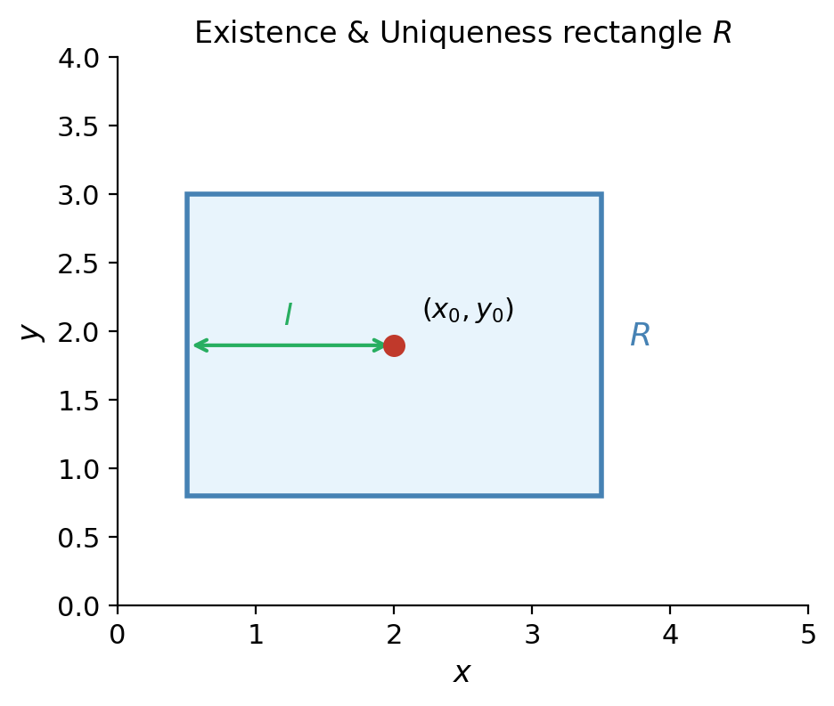
Notice three things. First, the theorem is local: it guarantees a solution on some interval around \(x_0\), which may be much smaller than the natural domain of \(f\). Second, continuity of \(f\) alone gives existence; continuity of \(\partial f / \partial y\) upgrades this to uniqueness. Third, if either condition fails, all bets are off: there may be no solution, infinitely many solutions, or a solution that blows up in finite time.
For the equation \(y' = 2x\sqrt{y}\) with \(y(0)=0\), the function \(f = 2x\sqrt{y}\) is continuous near \((0,0)\) but \(\partial f/\partial y = x/\sqrt{y}\) is not. Indeed, the IVP has two solutions: \(y \equiv 0\) and \(y = (x^2-c)^2\) for appropriate \(c\), illustrating that the uniqueness hypothesis cannot be dropped.
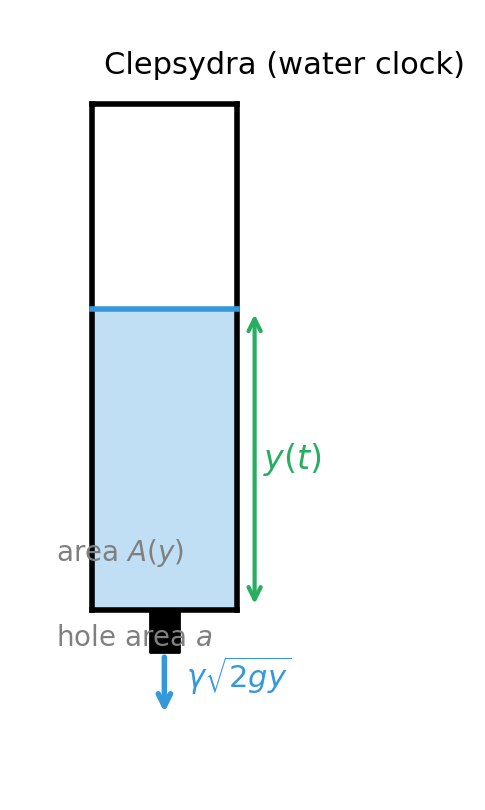
The draining clepsydra (water clock) is a physical instance of this: the height \(y(t)\) of water above a small outlet hole satisfies \(y' = -k\sqrt{y}\) (Torricelli’s law), so \(y=0\) is an equilibrium that the system can reach in finite time.
1.4 Classification of Differential Equations
It is worth collecting the taxonomy introduced above:
| Criterion | Categories |
|---|---|
| Number of independent variables | ODE / PDE |
| Order | 1st, 2nd, \(n\)th |
| Linearity | Linear / Nonlinear |
| Homogeneity (linear only) | Homogeneous / Nonhomogeneous |
| Coefficients (linear only) | Constant coefficients / Variable coefficients |
This classification determines which solution techniques apply. Constant-coefficient linear ODEs admit the characteristic-equation approach (Chapter 5). Variable-coefficient linear ODEs of order 2 can be attacked by reduction of order or power-series methods. Nonlinear ODEs often require qualitative or numerical methods.
Chapter 2: First-Order Ordinary Differential Equations
2.1 Geometry of First-Order Equations: Slope Fields
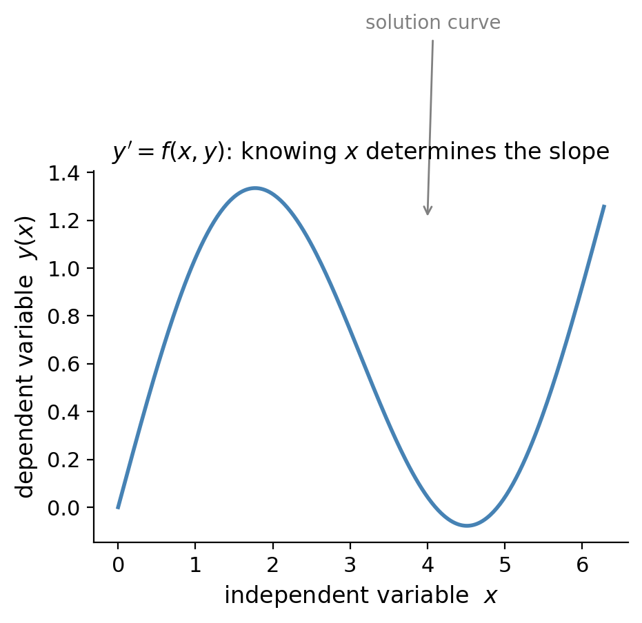
A first-order ODE \(y' = f(x,y)\) assigns to every point \((x,y)\) in the plane a slope \(f(x,y)\). Plotting a short line segment of that slope at a grid of points produces the slope field (or direction field) of the equation. Any solution curve must be tangent to the field at every point it passes through, so the slope field gives an immediate visual picture of all solutions simultaneously — without solving anything.
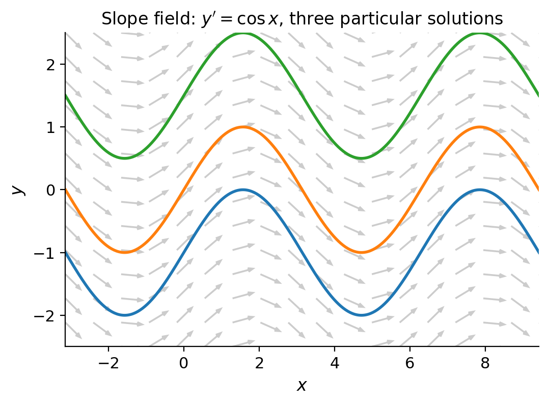
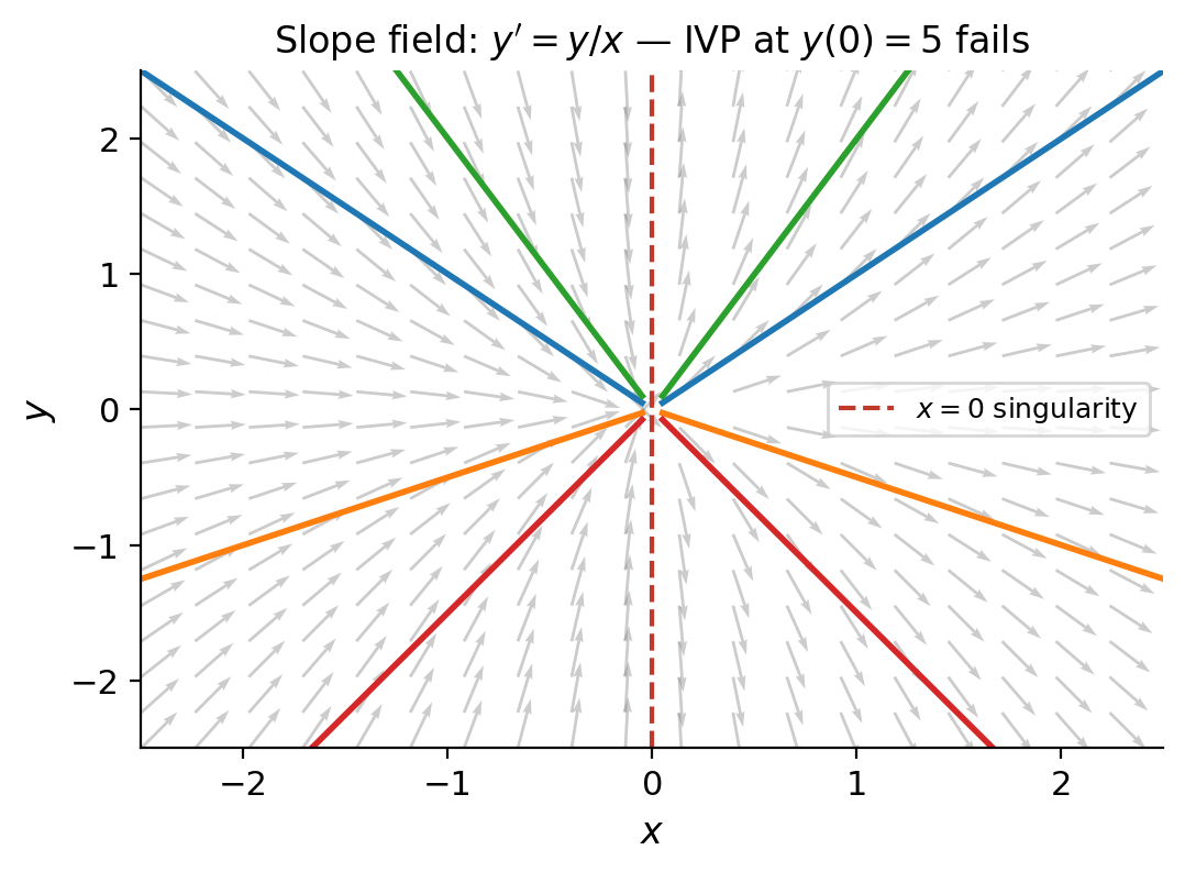
Slope fields reveal qualitative behavior that might be invisible in a formula. For example, the slope field for \(y' = y/x\) shows that every non-constant solution passes through the origin — but precisely there, both \(f\) and \(\partial f/\partial y\) blow up, so the E/U theorem does not apply and uniqueness fails.
2.2 Existence and Uniqueness for First-Order IVPs
The E/U theorem stated in Section 1.3 is illustrated sharply by the equation \(y' = 2\sqrt{y}\), \(y(0)=0\). Here \(f(x,y) = 2\sqrt{y}\) is continuous but \(\partial f/\partial y = 1/\sqrt{y}\) is not continuous at \(y=0\). Both \(y\equiv 0\) and \(y = (x-c)^2\) (for \(c>0\)) for appropriate piecewise definition satisfy the IVP, producing infinitely many solutions through the origin.
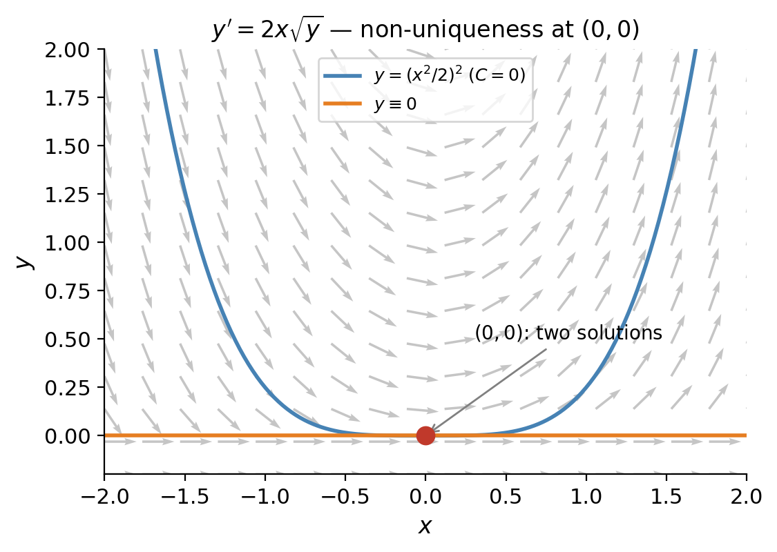
This example is not pathological: it models the draining of a tank (Torricelli’s law), so non-uniqueness has a physical interpretation — a dry tank stays dry, but also can spontaneously begin filling in reverse-time.
2.3 Exact Equations and the Criterion of Equality of Mixed Partials
A first-order ODE can be written in the differential form \(M(x,y)\,dx + N(x,y)\,dy = 0\). If there exists a function \(F(x,y)\) such that \(\partial F/\partial x = M\) and \(\partial F/\partial y = N\), the equation is called exact, and the general solution is the level set \(F(x,y)=C\).
The test for exactness is the equality of mixed partials: the equation is exact if and only if \(\partial M/\partial y = \partial N/\partial x\) on a simply-connected region. This follows from Clairaut’s theorem: if such an \(F\) exists, then \(\partial M/\partial y = \partial^2 F/\partial y\partial x = \partial^2 F/\partial x \partial y = \partial N/\partial x\).
To find \(F\) when the equation is exact: integrate \(M\) with respect to \(x\) holding \(y\) fixed to get a candidate \(F(x,y) = \int M\,dx + g(y)\), then differentiate with respect to \(y\) and match to \(N\) to determine \(g'(y)\), and hence \(g(y)\).
If the left side is a function of \(x\) alone — call it \(R(x)\) — then \(\mu(x)=e^{\int R(x)\,dx}\) is the integrating factor and the equation becomes exact. An analogous procedure works for integrating factors of the form \(\mu(y)\).
2.4 Separable Equations
\[\frac{dy}{h(y)} = g(x)\,dx\]and integrating both sides (using the implicit function theorem to justify the separation). The result is \(H(y) = G(x) + C\) where \(H'(y) = 1/h(y)\) and \(G'(x)=g(x)\). Solving for \(y\) may or may not be possible explicitly.
An important special case: if \(h(y) = y\), the equation \(y' = g(x)y\) is linear and separable. The solution is \(y = e^{G(x)+C} = Ae^{G(x)}\), which we will see again via the integrating factor method.
Separable equations also include autonomous equations \(y' = h(y)\) (no explicit \(x\) dependence). For autonomous equations, the long-run behavior is determined by equilibria — constant solutions where \(h(y^*)=0\). An equilibrium is stable if nearby solutions approach it as \(t\to\infty\); unstable if they move away. The sign of \(h(y)\) between equilibria tells you the direction of motion on the phase line (a number line for \(y\) with arrows showing whether \(y\) is increasing or decreasing). This graphical tool gives the full qualitative picture without solving the ODE.
2.5 Natural Growth and Decay
The simplest ODE model of a changing quantity is \(dP/dt = kP\): the rate of change is proportional to the current amount. This is both separable and linear. Separating variables and integrating: \(\int dP/P = \int k\,dt\), giving \(\ln|P| = kt + C\), so \(P(t) = P_0 e^{kt}\). If \(k>0\) the quantity grows exponentially; if \(k<0\) it decays.
This single model recurs in many guises:
- Radioactive decay: each atom has a fixed probability of decaying per unit time, giving \(N' = -\lambda N\). The half-life is \(t_{1/2} = \ln 2/\lambda\), the time for half the atoms to decay, independent of how many there are.
- Compound interest: \(dA/dt = rA\) where \(r\) is the annual rate. A deposit grows by a factor of \(e\) every \(1/r\) years.
- Mixing tanks and drug clearance: if a drug is eliminated at rate proportional to its concentration in the blood, the concentration decays exponentially — a fundamental assumption in pharmacokinetics.
The key insight is that rate proportional to amount and exponential function are two descriptions of the same phenomenon. Any time you see one, you should expect the other.
2.6 Linear First-Order Equations and the Integrating Factor
A first-order linear ODE is \(y' + P(x)y = Q(x)\). The technique of integrating factors was invented by Euler in 1734. The obstruction to direct integration is the \(P(x)y\) term: if only the left side looked like a derivative of a product, we could integrate immediately. The reverse product rule says \(d(\mu y)/dx = \mu' y + \mu y'\). We want this to equal \(\mu(y' + Py)\), which requires \(\mu' = \mu P(x)\) — a separable ODE for \(\mu\) itself, with solution \(\mu(x) = e^{\int P(x)\,dx}\). This choice of \(\mu\) is the integrating factor.
\[\mu(x)\,y = \int \mu(x)\,Q(x)\,dx + C \implies y = \frac{1}{\mu(x)}\left[\int \mu(x)Q(x)\,dx + C\right].\]The general solution always contains exactly one arbitrary constant, consistent with what the E/U theorem predicts for a first-order linear IVP.
2.7 Change of Variables: Homogeneous and Bernoulli Equations
Some first-order equations are not linear or separable as written, but become so after a substitution.
Homogeneous equations have the form \(y' = F(y/x)\). The substitution \(v = y/x\) (so \(y = vx\), \(y' = v + xv'\)) converts the equation to a separable ODE in \(v\) and \(x\).
Bernoulli equations have the form \(y' + P(x)y = Q(x)y^n\) (\(n \neq 0,1\)). Dividing by \(y^n\) gives \(y^{-n}y' + P(x)y^{1-n} = Q(x)\). The substitution \(w = y^{1-n}\) makes \(w' = (1-n)y^{-n}y'\), converting the equation to \(w'/(1-n) + P(x)w = Q(x)\) — a linear equation for \(w\).
These substitutions are not arbitrary tricks: they reflect genuine symmetry in the equation. The homogeneous substitution works because \(F(y/x)\) is invariant under rescaling \((x,y) \mapsto (\lambda x, \lambda y)\).
2.8 Reduction of Order: Second-Order Equations Missing y or x
Missing \(y\): If \(y\) does not appear explicitly, \(F(x,y',y'')=0\), the substitution \(p=y'\) (so \(y''=p'\)) reduces the equation to a first-order ODE \(F(x,p,p')=0\). Solve for \(p(x)\), then integrate to get \(y = \int p\,dx + C\).
Missing \(x\): If \(x\) does not appear explicitly, \(F(y,y',y'')=0\), treat \(p=y'\) as a function of \(y\). By the chain rule, \(y'' = dp/dx = (dp/dy)(dy/dx) = p\,dp/dy\). The equation becomes \(F(y,p,p\,dp/dy)=0\), a first-order ODE in \(p\) as a function of \(y\).
These reductions are the simplest examples of a broader theme: whenever a symmetry or conservation law is present — here translational symmetry in \(y\) (first case) or in \(x\) (second case) — the order of the ODE can be reduced by one.
Chapter 3: Mathematical Models and Numerical Methods
3.1 Population Models — Logistic Growth, Equilibria, Stability
\[\frac{dP}{dt} = kP\left(1 - \frac{P}{K}\right),\]where \(K > 0\) is the carrying capacity. The factor \((1-P/K)\) reduces the growth rate as \(P\) approaches \(K\), modeling resource limitation.
\[\frac{dP}{P(1-P/K)} = k\,dt \implies \left(\frac{1}{P}+\frac{1/K}{1-P/K}\right)dP = k\,dt.\]\[P(t) = \frac{KP_0}{P_0 + (K-P_0)e^{-kt}}.\]The long-term behavior is determined by two equilibria:
- \(P^* = 0\): the extinction state (unstable if \(k>0\)).
- \(P^* = K\): the carrying capacity (asymptotically stable if \(k>0\)).
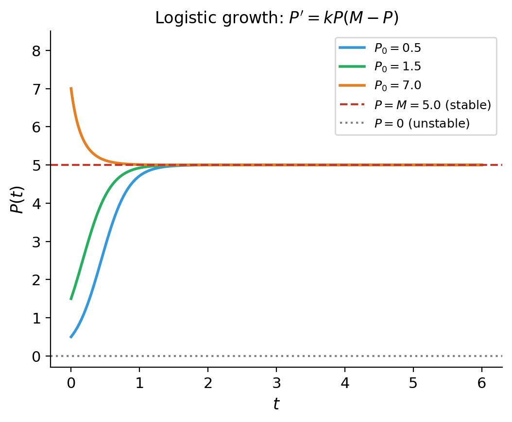
Phase-line analysis captures this without solving: plot \(dP/dt\) vs \(P\). Where \(dP/dt > 0\), \(P\) is increasing; where \(dP/dt < 0\), \(P\) is decreasing. Arrows on the phase line immediately reveal that \(P=0\) is unstable and \(P=K\) is stable.
3.2 Logistic Growth with Harvesting and Bifurcation
\[\frac{dP}{dt} = kP\left(1 - \frac{P}{K}\right) - h.\]Equilibria satisfy a quadratic in \(P\). For small \(h\) there are two positive equilibria; as \(h\) increases, they collide at a saddle-node bifurcation and disappear, leaving no positive equilibrium — extinction is then inevitable regardless of initial population. The critical harvest rate is \(h^* = kK/4\).
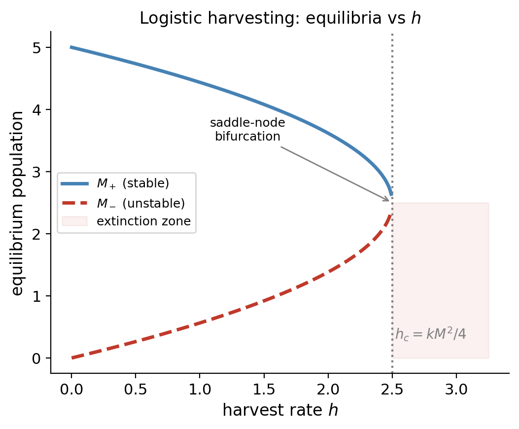
This is a canonical example in bifurcation theory: a qualitative change in the structure of equilibria as a parameter crosses a threshold. Strogatz dedicates substantial discussion to this scenario as the simplest route to understanding catastrophic collapse in ecological, economic, and engineering systems.
3.3 Newton’s Law of Cooling
\[\frac{dT}{dt} = -k(T - T_\infty), \quad k > 0.\]\[T(t) = T_\infty + (T_0 - T_\infty)e^{-kt}.\]The temperature difference decays exponentially to zero, regardless of the sign of \(T_0 - T_\infty\) — a hot object cools and a cold object warms. The rate constant \(k\) depends on the object’s surface area, heat capacity, and the convection properties of the surrounding medium.
From \(T(10) = 70\): \(70 = 20 + 70e^{-10k}\), so \(e^{-10k} = 50/70 = 5/7\), giving \(k = \tfrac{1}{10}\ln(7/5)\). Now solve \(40 = 20 + 70e^{-kt}\): \(e^{-kt} = 2/7\), so \(t = \ln(7/2)/k = 10\ln(7/2)/\ln(7/5) \approx 43\) minutes.
3.4 Position–Velocity Models with Air Resistance
\[m\frac{dv}{dt} = mg - cv.\]\[v(t) = \frac{mg}{c} + \left(v_0 - \frac{mg}{c}\right)e^{-ct/m}.\]The terminal velocity \(v_\infty = mg/c\) is the equilibrium: as \(t\to\infty\), \(v(t)\to v_\infty\) regardless of initial velocity.
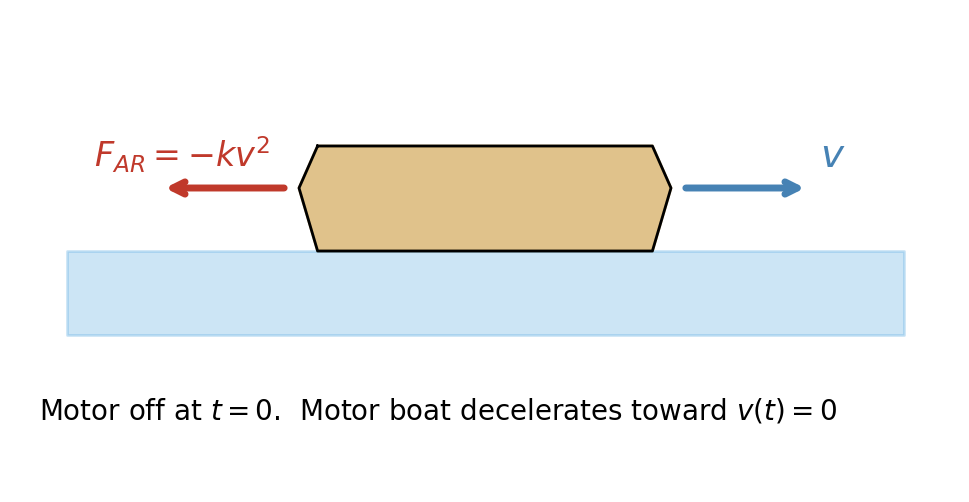
For a boat decelerating against resistance proportional to \(v^2\) (\(F = -kv^2\)), the equation becomes \(mv' = -kv^2\), which is separable. Separating: \(dv/v^2 = -(k/m)\,dt\), integrating: \(-1/v = -(k/m)t + C\), so \(v(t) = mv_0/(m + kv_0 t)\). The velocity decreases like \(1/t\) — much more slowly than the exponential decay from linear resistance, so the boat glides a long way before stopping.
3.5 Newton’s Law of Gravitation and Escape Velocity
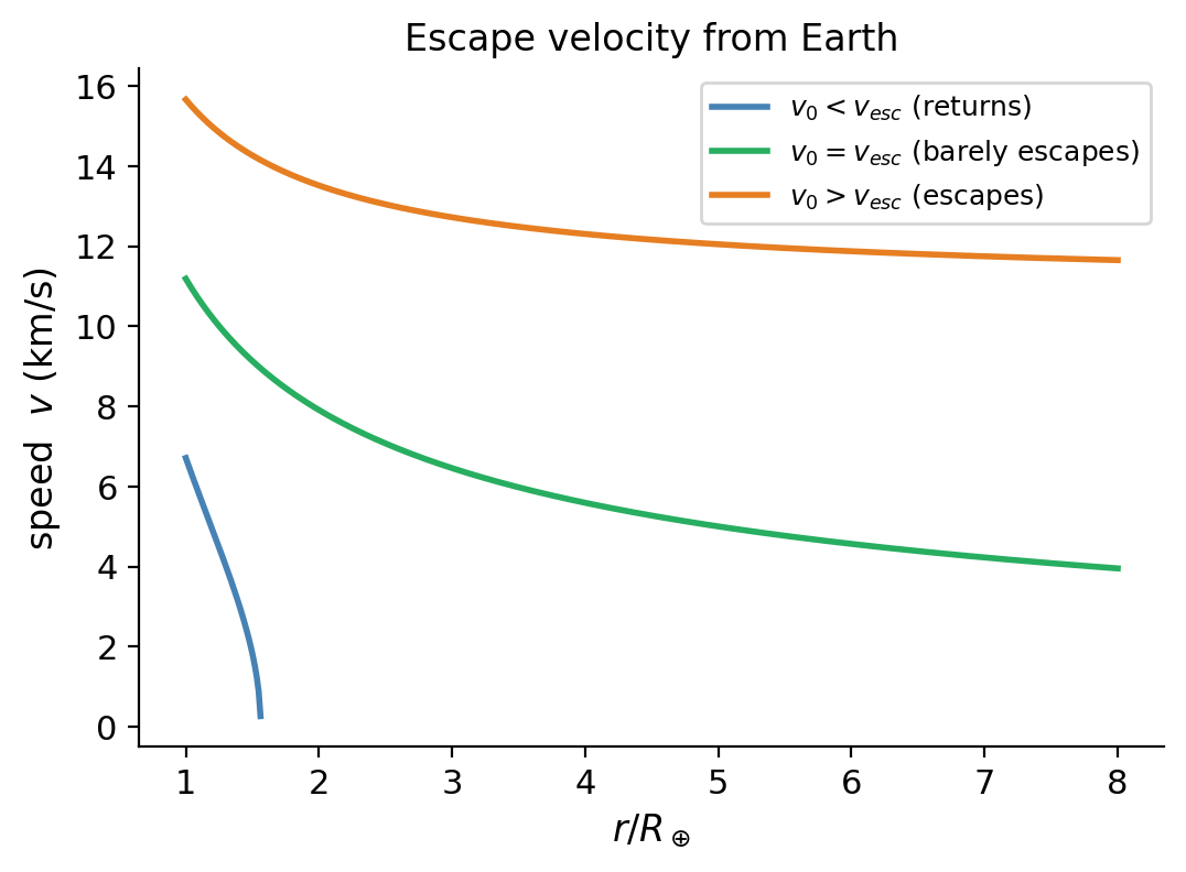
\[m\frac{d^2r}{dt^2} = -\frac{GMm}{r^2}.\]\[mv\frac{dv}{dr} = -\frac{GMm}{r^2}.\]Integrating: \(\frac{1}{2}v^2 = \frac{GM}{r} + C\). Applying \(v(R)=v_0\) determines \(C\). Escape occurs if \(v\) remains positive for all \(r>R\), which requires \(\frac{1}{2}v_0^2 \geq GM/R\). Thus the escape velocity is \(v_{\mathrm{esc}} = \sqrt{2GM/R} \approx 11.2\) km/s for Earth.
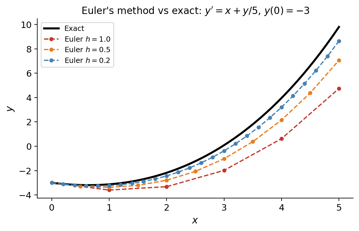
3.6 Euler’s Method and Sources of Error
\[x_{n+1} = x_n + h, \quad y_{n+1} = y_n + h\cdot f(x_n, y_n).\]At each step, the solution curve is approximated by its tangent line. The local truncation error at each step is \(O(h^2)\), and accumulating over \(N = (b-a)/h\) steps gives a global error of \(O(h)\). Halving the step size halves the error — Euler’s method is first-order accurate.
Two sources of error matter in practice:
- Truncation error: error from replacing the ODE by a finite difference approximation.
- Round-off error: accumulation of floating-point arithmetic errors. Reducing \(h\) reduces truncation error but eventually increases round-off error, so there is an optimal step size.
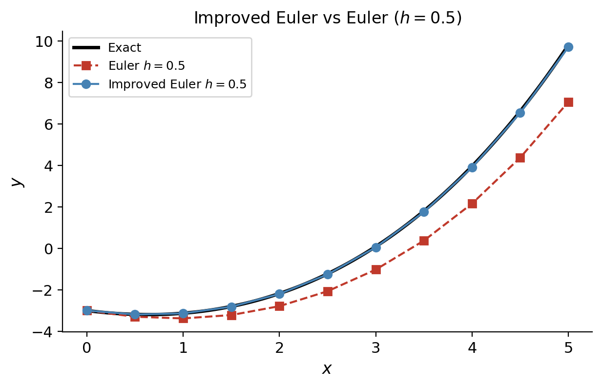
3.7 The Improved Euler Method
\[\tilde{y}_{n+1} = y_n + h\cdot f(x_n, y_n) \quad \text{(predictor)}\]\[y_{n+1} = y_n + \frac{h}{2}\left[f(x_n,y_n) + f(x_{n+1},\tilde{y}_{n+1})\right] \quad \text{(corrector).}\]The global error is \(O(h^2)\), so this is a second-order method. The improvement over basic Euler is substantial in practice.
3.8 Proof Sketch of the Existence–Uniqueness Theorem (Picard Iteration)
\[y(x) = y_0 + \int_{x_0}^x f(t, y(t))\,dt,\]\[y_{n+1}(x) = y_0 + \int_{x_0}^x f(t, y_n(t))\,dt.\]Under the hypotheses of the theorem (Lipschitz continuity of \(f\) in \(y\)), this sequence converges uniformly to a solution.
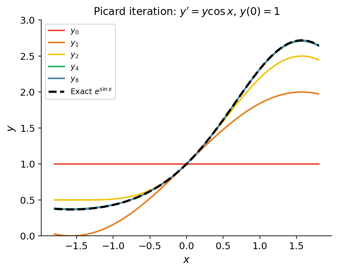
The proof uses the Banach fixed-point theorem (contraction mapping principle): the operator \(T[y](x) = y_0 + \int_{x_0}^x f(t,y(t))\,dt\) is a contraction on a suitable function space, so it has a unique fixed point — the solution.
Chapter 4: Dimensional Analysis
4.1 Fundamental Quantities and the Principle of Dimensional Homogeneity
Before writing down any differential equation to model a physical system, it is worth asking: what are the relevant quantities, and how do they relate dimensionally? This is the subject of dimensional analysis, a powerful technique that can yield qualitative information — and sometimes the full functional form of a relationship — without solving any equations.
Every physical quantity has a dimension that can be expressed in terms of the fundamental quantities: mass \([M]\), length \([L]\), time \([T]\), temperature \([\Theta]\), and so on. The Principle of Dimensional Homogeneity says: every term in a valid physical equation must have the same dimensions. This principle, simple as it sounds, is remarkably constraining.
\[V\frac{dC}{dt} = QC_{\mathrm{in}} - QC\](volume \(V\), flow rate \(Q\), concentration \(C\)), define dimensionless time \(\tau = Qt/V\) and dimensionless concentration \(c = C/C_{\mathrm{in}}\). The equation becomes simply \(dc/d\tau = 1 - c\), containing no parameters at all. The single dimensionless group \(\tau = Qt/V\) — the number of “tank volumes” that have flowed through — captures all the physics.
4.2 The Buckingham π Theorem
When a physical relationship involves \(n\) dimensional quantities and \(k\) independent fundamental dimensions, the relationship can be expressed in terms of \(n-k\) dimensionless groups (called π-groups). This is the Buckingham π Theorem, published in 1914 (though anticipated by Lord Rayleigh).
The theorem does not tell you which dimensionless groups to form — that requires physical insight — but it tells you how many there are. Reducing the number of parameters from \(n\) to \(n-k\) collapses the parameter space and makes experiments far more efficient.
4.3 Worked Example: The Pendulum Period
\[\pi_1 = T\sqrt{g/\ell}, \qquad \pi_2 = \theta_0.\]\[T = C\sqrt{\frac{\ell}{g}}\]for some universal constant \(C\). The full solution of the linearized ODE gives \(C = 2\pi\).
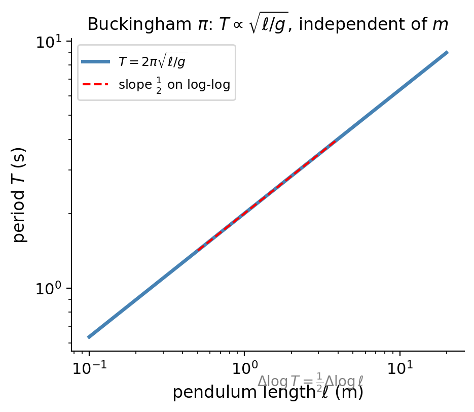
This result — that the period is independent of mass and proportional to \(\sqrt{\ell}\) — was discovered experimentally by Galileo around 1602, long before any ODE was written down. Dimensional analysis gives it in three lines.
Chapter 5: Linear Equations of Higher Order
5.1 The Linear Operator and the Superposition Principle
\[L[y] = y^{(n)} + P_1(x)y^{(n-1)} + \cdots + P_n(x)y.\]The adjective “linear” here has a precise meaning: \(L[\alpha y_1 + \beta y_2] = \alpha L[y_1] + \beta L[y_2]\) for any constants \(\alpha, \beta\) and functions \(y_1, y_2\). This algebraic property is what makes the theory tractable.
Moreover, if \(y_p\) is any particular solution of the nonhomogeneous equation \(L[y]=f(x)\) and \(y_h\) is the general solution of the associated homogeneous equation \(L[y]=0\), then the general solution of \(L[y]=f(x)\) is \(y = y_h + y_p\). This complementary function + particular integral structure is the backbone of all linear ODE theory.
The existence, uniqueness, and structure of solutions for higher-order linear IVPs mirror the first-order theory exactly.
Just as for first-order systems, the key point is global existence on the full interval of continuity — not just locally near \(x_0\). This is the dividend of linearity.
5.2 The Wronskian, Linear Independence, and Abel’s Identity
To determine whether \(n\) solutions span the full solution space, we need a test for linear independence.
This dichotomy — either always zero or never zero — is special to solutions of a linear ODE and does not hold for arbitrary functions. It is a consequence of Abel’s identity.
In particular, \(W\) satisfies the first-order linear ODE \(W' = -P_1(x)W\), so it is either identically zero or never zero. For the second-order case this is Liouville’s formula.
A set of \(n\) linearly independent solutions is called a fundamental set of solutions, and the general solution is then \(y = c_1 y_1 + \cdots + c_n y_n\).
5.3 Homogeneous Equations with Constant Coefficients — The Characteristic Equation
\[a_n y^{(n)} + a_{n-1}y^{(n-1)} + \cdots + a_1 y' + a_0 y = 0\]\[L[e^{rx}] = e^{rx}(a_n r^n + a_{n-1}r^{n-1} + \cdots + a_1 r + a_0) = p(r)\,e^{rx}.\]For \(e^{rx}\) to be a solution we need \(L[e^{rx}]=0\), i.e. \(p(r)=0\). The roots of \(p(r)=0\) (the characteristic equation), counting multiplicity and allowing complex values, completely determine the solution space by the General Solution Theorem.
5.4 Real, Repeated, and Complex Roots
The three cases for the characteristic roots are:
Case 1: Distinct real roots \(r_1, r_2, \ldots, r_n\). Solutions: \(e^{r_1 x}, e^{r_2 x}, \ldots, e^{r_n x}\). The Wronskian is a Vandermonde determinant times \(e^{(r_1+\cdots+r_n)x}\), which is nonzero when all \(r_i\) are distinct.
Case 2: Repeated real root \(r\) with multiplicity \(m\). Solutions: \(e^{rx}, xe^{rx}, x^2e^{rx}, \ldots, x^{m-1}e^{rx}\). The polynomial prefactors are found by reduction of order: given the known solution \(e^{rx}\), substitute \(y = u(x)e^{rx}\) into the ODE. Because \(r\) is a root of multiplicity \(m\), the equation for \(u\) reduces to \(u^{(m)}=0\), whose general solution is a polynomial of degree \(m-1\), producing exactly the \(m\) solutions listed.
Case 3: Complex conjugate roots \(\alpha \pm i\beta\) (simple). By Euler’s formula \(e^{(\alpha\pm i\beta)x} = e^{\alpha x}(\cos\beta x \pm i\sin\beta x)\), taking real and imaginary parts gives two real solutions: \(e^{\alpha x}\cos\beta x\) and \(e^{\alpha x}\sin\beta x\). If the complex root has multiplicity \(m\), multiply each by \(1, x, x^2, \ldots, x^{m-1}\).
5.5 The Mass–Spring System: Free Undamped, Underdamped, Critically Damped, Overdamped
\[mx'' + cx' + kx = 0.\]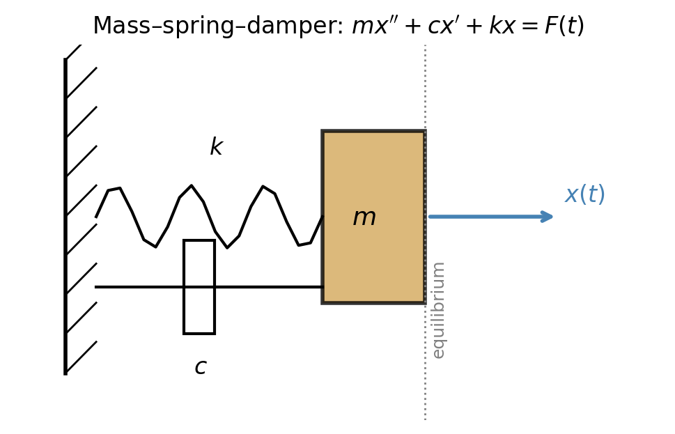
Set \(\omega_0 = \sqrt{k/m}\) (natural frequency) and \(\gamma = c/(2m)\) (damping coefficient). The characteristic equation is \(r^2 + 2\gamma r + \omega_0^2 = 0\), with roots \(r = -\gamma \pm \sqrt{\gamma^2 - \omega_0^2}\).
Free undamped (\(c=0\), \(\gamma=0\)): roots \(r = \pm i\omega_0\). Solution \(x = A\cos(\omega_0 t - \phi)\), simple harmonic motion with period \(2\pi/\omega_0\).
Underdamped (\(c^2 < 4km\), i.e. \(\gamma < \omega_0\)): complex roots \(-\gamma \pm i\omega_d\) where \(\omega_d = \sqrt{\omega_0^2 - \gamma^2}\) is the damped natural frequency. Solution \(x = Ae^{-\gamma t}\cos(\omega_d t - \phi)\): oscillations with exponentially decaying amplitude.
Critically damped (\(c^2 = 4km\)): repeated real root \(r = -\gamma\). Solution \(x = (c_1 + c_2 t)e^{-\gamma t}\): fastest non-oscillatory return to equilibrium.
Overdamped (\(c^2 > 4km\)): two distinct negative real roots. Solution is a sum of two decaying exponentials; the return to equilibrium is slower than critical damping.
The distinction matters in engineering: door closers are designed to be slightly overdamped; vehicle suspensions aim for slight underdamping for comfort.
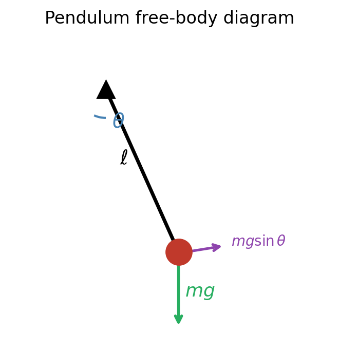
5.6 The Pendulum: Linearization and Free Oscillations
\[\theta'' + \frac{g}{\ell}\theta = 0, \quad \theta(0)=\theta_0, \quad \theta'(0)=v_0.\]This is the free undamped harmonic oscillator with \(\omega_0 = \sqrt{g/\ell}\). The period \(T = 2\pi\sqrt{\ell/g}\) is independent of amplitude — the isochrony of the pendulum, which Galileo famously observed by timing his own pulse against a swinging chandelier in Pisa around 1602.
The linearization is valid only for \(|\theta| \lesssim 15^\circ\); beyond that, the period increases noticeably. For large amplitudes the motion is still periodic but not sinusoidal, and the period must be computed via elliptic integrals.
5.7 Non-homogeneous Equations: Method of Undetermined Coefficients
For a constant-coefficient nonhomogeneous equation \(L[y]=f(x)\) where \(f(x)\) is a combination of polynomials, exponentials, sines, and cosines (or products thereof), the method of undetermined coefficients seeks a particular solution of the same “type” as \(f\).
\[y_p = x^s e^{\alpha x}(P_m(x)\cos\beta x + Q_m(x)\sin\beta x)\]where \(P_m, Q_m\) are polynomials of degree \(m\) to be determined, and \(s=0\) if \(\alpha + i\beta\) is not a root of the characteristic polynomial, \(s=1\) if it is a simple root, \(s=2\) if it is a double root, and so on. The factor \(x^s\) is the crucial modification rule: it prevents the trial particular solution from being a solution of the homogeneous equation, which would make substitution give 0=0 and determine nothing.
5.8 Variation of Parameters
When undetermined coefficients cannot be applied — because the right-hand side \(f(x)\) is not of the standard polynomial-exponential-trigonometric type, or because the coefficients are variable — we use variation of parameters, a general method applicable to any \(n\)th-order linear ODE.
\[y_p' = y_1'u_1 + y_2'u_2 + y_1 u_1' + y_2 u_2'.\]\[y_p'' = y_1''u_1 + y_2''u_2 + y_1'u_1' + y_2'u_2'.\]\[y_1' u_1' + y_2' u_2' = f.\]\[u_1'(x) = -\frac{y_2(x)f(x)}{W(x)}, \qquad u_2'(x) = \frac{y_1(x)f(x)}{W(x)},\]where \(W = W(y_1,y_2)\) is the Wronskian.
5.9 Forced Oscillations: Resonance and Beats (Undamped)
\[x'' + \omega_0^2 x = A_0\cos(\omega t), \quad x(0)=0,\; x'(0)=0,\]where \(\omega_0 = \sqrt{k/m}\) is the natural frequency and \(\omega\) is the forcing frequency.
\[x(t) = \frac{F_0}{m(\omega_0^2 - \omega^2)}(\cos\omega t - \cos\omega_0 t).\]\[x(t) = \frac{2F_0}{m(\omega_0^2-\omega^2)}\sin\!\left(\frac{\omega_0-\omega}{2}t\right)\sin\!\left(\frac{\omega_0+\omega}{2}t\right).\]When \(\omega\) is close to \(\omega_0\), the factor \((\omega_0-\omega)/2\) is small, producing a slowly varying envelope around the rapid oscillation at frequency \((\omega_0+\omega)/2 \approx \omega_0\). This is beating: the amplitude oscillates at the beat frequency \(|\omega_0-\omega|\).
The amplitude grows linearly without bound — pure resonance. In physical terms, each cycle of the forcing input adds energy to the system, and with no damping to remove energy, the amplitude grows indefinitely.
Pure resonance is the reason soldiers are ordered to break step when crossing a bridge: the rhythmic forcing of a marching column could theoretically match the bridge’s natural frequency. The 1850 collapse of the Angers suspension bridge in France killed 226 soldiers for exactly this reason.
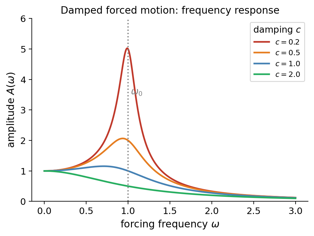
5.10 Damped Forced Motion and Frequency Response
\[mx'' + cx' + kx = F_0\cos(\omega t).\]\[x_p(t) = \frac{F_0/m}{\sqrt{(\omega_0^2-\omega^2)^2+4\gamma^2\omega^2}}\cos(\omega t - \phi),\]\[C(\omega) = \frac{F_0/m}{\sqrt{(\omega_0^2-\omega^2)^2+4\gamma^2\omega^2}}.\]Plotting \(C(\omega)\) vs \(\omega\) gives the frequency response curve. For small damping (\(\gamma \ll \omega_0\)) there is a sharp peak near \(\omega = \omega_0\); for large damping the peak flattens out. The resonant frequency shifts to \(\omega_r = \sqrt{\omega_0^2 - 2\gamma^2}\) (slightly below \(\omega_0\) for small \(\gamma\)), and the maximum amplitude is approximately \(F_0/(2m\gamma\omega_0)\).
Chapter 6: Linear Systems of ODEs
6.1 Matrix Formulation and the Existence–Uniqueness Theorem for Systems
\[\begin{pmatrix}x_1'\\x_2'\end{pmatrix} = \begin{pmatrix}0&1\\-k/m&-c/m\end{pmatrix}\begin{pmatrix}x_1\\x_2\end{pmatrix}+\begin{pmatrix}0\\F(t)/m\end{pmatrix}.\]The general first-order linear system takes the form \(\vec{x}' = P(t)\vec{x} + \vec{f}(t)\), where \(P(t)\) is an \(n\times n\) matrix of coefficient functions and \(\vec{f}(t)\) is a vector of forcing terms.
Notice the key difference from the scalar case: the solution exists globally on the entire interval of continuity of the coefficients, not just locally near \(t_0\). For linear systems there is no finite-time blowup — the solution is as long-lived as the coefficients are well-behaved.
The structure of solutions parallels the scalar theory: the general solution of the homogeneous system \(\vec{x}'=P(t)\vec{x}\) is a linear combination of \(n\) linearly independent solutions (a fundamental set), and the general solution of the nonhomogeneous system adds any particular solution.
6.2 The Eigenvalue Method for Constant-Coefficient Homogeneous Systems
\[\lambda e^{\lambda t}\vec{v} = Ae^{\lambda t}\vec{v} \implies A\vec{v} = \lambda\vec{v}.\]So \(\lambda\) must be an eigenvalue of \(A\) and \(\vec{v}\) the corresponding eigenvector. Eigenvalues are roots of the characteristic equation \(\det(A-\lambda I)=0\).
For a \(2\times 2\) system there are three cases, just as for a scalar second-order ODE:
\[\vec{x}(t) = c_1 e^{\lambda_1 t}\vec{v}_1 + c_2 e^{\lambda_2 t}\vec{v}_2.\]6.3 Sketching Solutions in the Phase Plane (2D Phase Portraits)
For a 2D system \(\vec{x}'=A\vec{x}\), a phase portrait is a representative collection of solution curves (trajectories) drawn in the \((x_1,x_2)\)-plane. Rather than plotting each component against time separately, we treat \((x_1(t),x_2(t))\) as a parametric curve — the trajectory of the state as time flows forward.
Consider \(A=\begin{pmatrix}0&1\\-1&0\end{pmatrix}\), which has eigenvalues \(\pm i\) and general solution \(\vec{x}(t)=c_1\binom{\cos t}{-\sin t}+c_2\binom{\sin t}{\cos t}\). For \(c_2=0\), \(x_1=a\cos t\) and \(x_2=-a\sin t\), parametrizing the circle \(x_1^2+x_2^2=a^2\). The phase portrait consists of concentric circles — a center.
For the saddle example \(A=\begin{pmatrix}1&1\\4&1\end{pmatrix}\) with \(\lambda=3,-1\):
- The eigenvectors define straight-line special solutions (called separatrices or eigenspaces).
- On the eigenvector for \(\lambda=3\), trajectories move outward; on that for \(\lambda=-1\), inward.
- All other trajectories are asymptotic to the \(\lambda=3\) eigenvector as \(t\to\infty\) and to the \(\lambda=-1\) eigenvector as \(t\to-\infty\).
Nullclines (where \(x_1'=0\) or \(x_2'=0\)) provide additional geometric landmarks:
- Vertical nullclines (\(x_1'=0\)): trajectories cross these horizontally.
- Horizontal nullclines (\(x_2'=0\)): trajectories cross these vertically.
6.4 Classification of Equilibria — Nodes, Saddles, Spirals, Centers
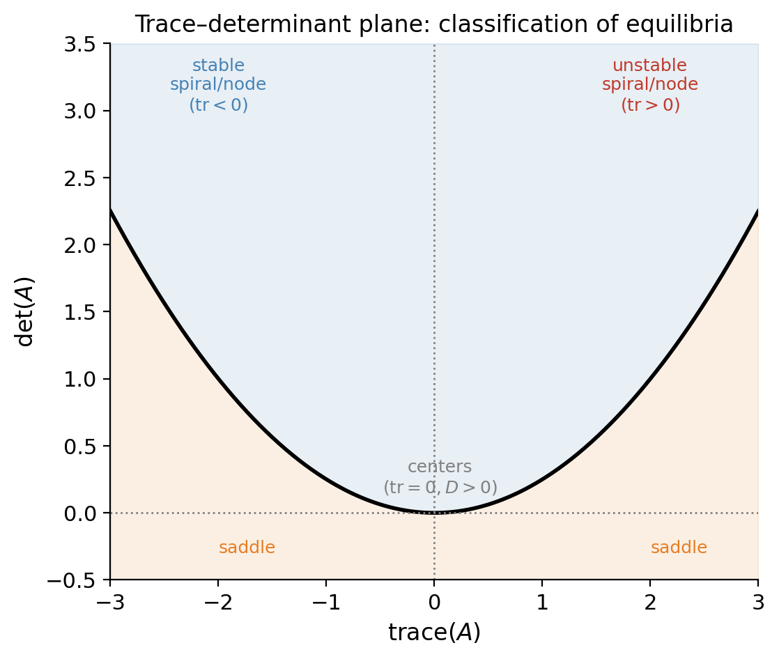
For the constant-coefficient system \(\vec{x}'=A\vec{x}\), the origin is always an equilibrium. Its character depends on the eigenvalues of \(A\):
| Eigenvalue Type | Portrait | Stability |
|---|---|---|
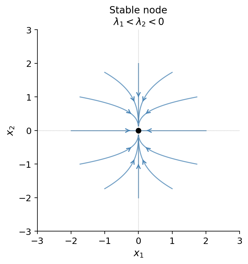
| \(\lambda_1 < \lambda_2 < 0\) (both negative) | Stable node | Asymptotically stable |
| \(0 < \lambda_1 < \lambda_2\) (both positive) | Unstable node | Unstable |
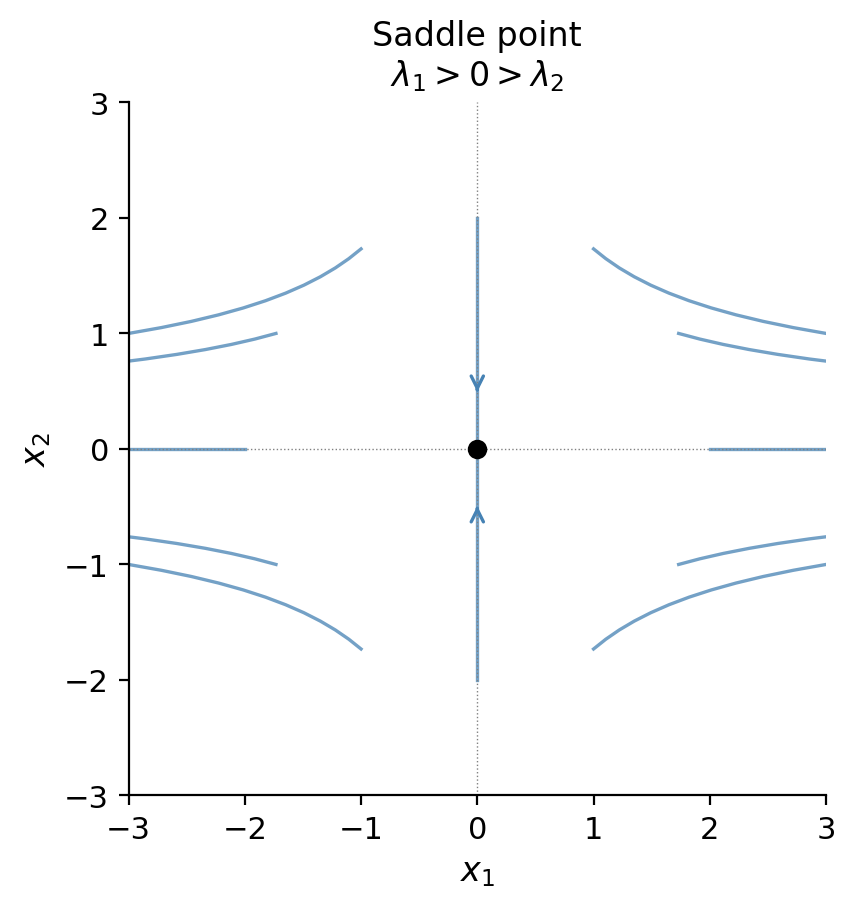
| \(\lambda_1 < 0 < \lambda_2\) (opposite signs) | Saddle | Unstable |
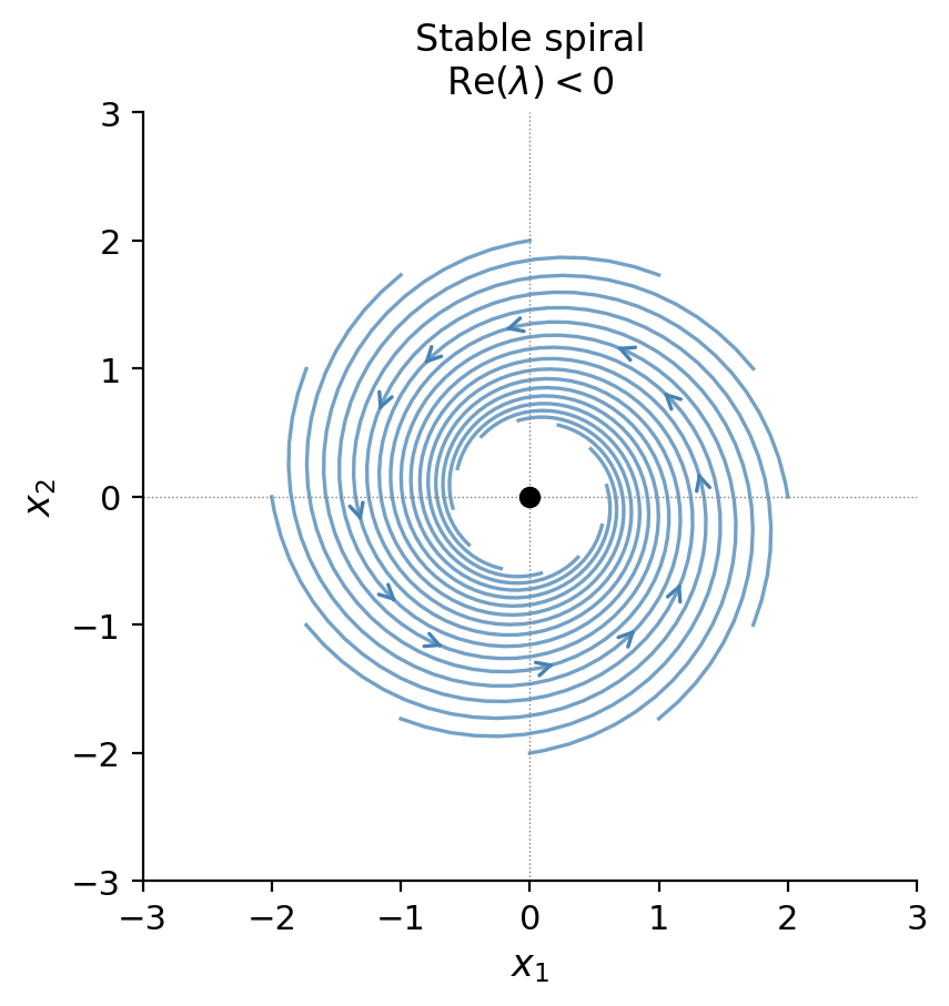
| \(\lambda = \alpha \pm i\beta\), \(\alpha < 0\) | Stable spiral | Asymptotically stable |
| \(\lambda = \alpha \pm i\beta\), \(\alpha > 0\) | Unstable spiral | Unstable |
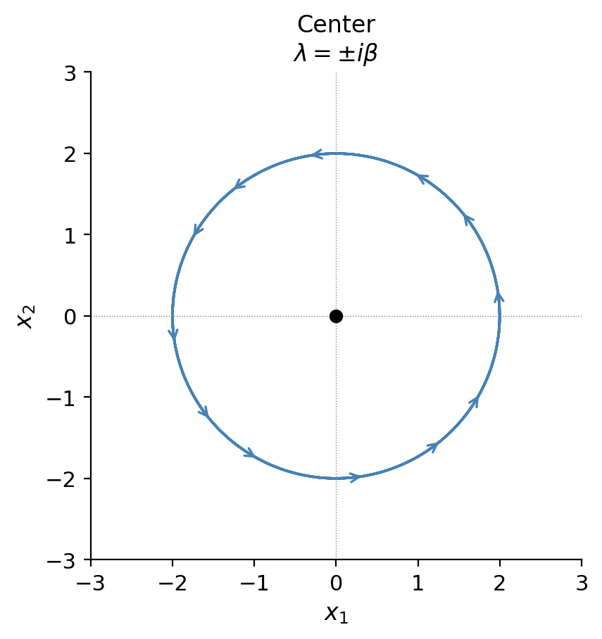
| \(\lambda = \pm i\beta\) (purely imaginary) | Center | Stable (not asymptotically) |
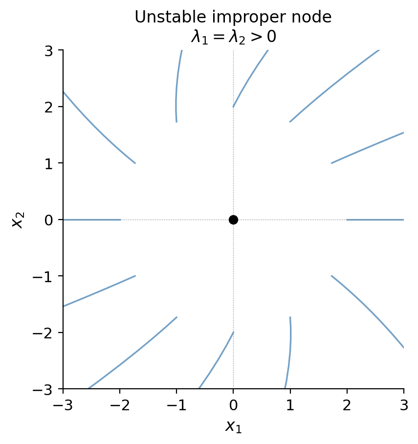
| \(\lambda_1=\lambda_2=\lambda<0\), defective | Stable improper node | Asymptotically stable |
The trace–determinant plane (plotting \(\tau = \text{tr}(A)\) on the horizontal axis and \(\Delta = \det(A)\) on the vertical axis) summarizes all cases geometrically: the boundary between spirals and nodes is the parabola \(\tau^2=4\Delta\); saddles live below the \(\tau\)-axis (\(\Delta<0\)); centers on the vertical axis (\(\tau=0, \Delta>0\)).
Stable node (\(\lambda_1 < \lambda_2 < 0\)): all trajectories approach the origin, asymptotically tangent to the eigenvector of the slower-decaying mode (the larger eigenvalue \(\lambda_2\)). The portrait shows curved arcs bending into that direction as \(t\to\infty\).
Saddle (\(\lambda_1 < 0 < \lambda_2\)): two straight separatrices, one along each eigenvector. Along the \(\lambda_1\)-eigenvector, trajectories flow into the origin; along \(\lambda_2\), they flow out. All other trajectories approach the outgoing separatrix as \(t\to\infty\) and came from the incoming one as \(t\to -\infty\). The origin is always unstable.
Stable spiral (\(\alpha < 0\)): the real part of the eigenvalue controls exponential decay; the imaginary part \(\beta\) controls the rotation rate. Trajectories wind inward, tightening into the origin. The direction of winding (clockwise or counter-clockwise) depends on the sign of \(\beta\) and the entries of \(A\).
Center (\(\alpha = 0\)): the decay vanishes exactly and trajectories are closed ellipses. This is the phase portrait of the undamped harmonic oscillator. It sits on the boundary between stable and unstable spirals; any perturbation of \(A\) that adds a real part to the eigenvalue destroys it.
Improper node (repeated eigenvalue \(\lambda < 0\), defective): there is only one eigenvector direction. Trajectories approach the origin tangent to it, but without the branching seen in the proper node case. This portrait arises precisely at the boundary between two distinct real eigenvalues and complex conjugate eigenvalues in the trace–determinant plane (the parabola \(\tau^2=4\Delta\)).
6.5 The Fundamental Matrix
The fundamental matrix has several key properties:
- \(\Phi\) satisfies the matrix ODE \(\Phi'(t) = P(t)\Phi(t)\), since each column satisfies the system.
- General solution: \(\vec{x}(t) = \Phi(t)\vec{c}\) for arbitrary \(\vec{c}\in\mathbb{R}^n\).
- Solution to IVP: If \(\Phi(t_0)=I\) (this is called the principal fundamental matrix at \(t_0\)), then the solution to \(\vec{x}'=P\vec{x}\), \(\vec{x}(t_0)=\vec{x}_0\) is \(\vec{x}(t)=\Phi(t)\vec{x}_0\).
- \(\Phi(t)\) is invertible for all \(t\in I\), since \(\det\Phi(t)\neq 0\).
- Abel’s identity in matrix form: \(\det\Phi(t)=\det\Phi(t_0)\exp\!\left(\int_{t_0}^t \text{tr}\,P(s)\,ds\right)\).
This is invertible for all \(t\) since \(\det\Phi(t) = e^{(\lambda_1+\lambda_2)t}\det\begin{pmatrix}v_{11}&v_{21}\\v_{12}&v_{22}\end{pmatrix}\neq 0\) when \(\vec{v}_1,\vec{v}_2\) are linearly independent.
For repeated or complex eigenvalues, the fundamental matrix is constructed from the corresponding Case 2 or Case 3 solutions. In all cases the structure is the same: \(\Phi(t)\) packages the general solution into a single matrix object, making it easy to apply arbitrary initial conditions by computing \(\vec{x}(t) = \Phi(t)\Phi(t_0)^{-1}\vec{x}_0\).
\[e^{At} = I + At + \frac{(At)^2}{2!} + \frac{(At)^3}{3!} + \cdots = \sum_{k=0}^\infty \frac{(At)^k}{k!},\]which converges for all \(t\) and all \(A\). The matrix exponential satisfies \(\frac{d}{dt}e^{At}=Ae^{At}\) and the semigroup property \(e^{A(t+s)}=e^{At}e^{As}\). The general solution of \(\vec{x}'=A\vec{x}\) is \(\vec{x}(t)=e^{At}\vec{x}_0\).
In practice, \(e^{At}\) is computed from the eigenvalue-method solutions: express the fundamental matrix \(\Phi(t)\) built from eigenvalue-method solutions (as above), then \(e^{At}=\Phi(t)\Phi(0)^{-1}\). For a diagonal matrix \(D=\text{diag}(\lambda_1,\ldots,\lambda_n)\), \(e^{Dt}=\text{diag}(e^{\lambda_1 t},\ldots,e^{\lambda_n t})\), and if \(A=PDP^{-1}\) then \(e^{At}=Pe^{Dt}P^{-1}\).
6.6 Non-homogeneous Linear Systems and Variation of Parameters
\[\vec{x}(t) = \underbrace{\Phi(t)\vec{c}}_{\vec{x}_h(t)} + \underbrace{\vec{x}_p(t)}_{\text{particular}}\]where \(\Phi(t)\) is a fundamental matrix for the associated homogeneous system. The variation of parameters method finds \(\vec{x}_p\) by allowing the constant vector \(\vec{c}\) to vary with \(t\).
General solution: \(\vec{x}(t)=\vec{x}_h(t)+\vec{x}_p(t)\).
Chapter 7: Laplace Transforms
7.1 Definition, Convergence, and Linearity
The Laplace transform is a way of converting a differential equation into an algebraic equation. Where classical solution methods require guessing solution forms and applying initial conditions at the end, the Laplace transform incorporates initial conditions at the start and reduces the ODE to algebra in the transform variable \(s\). This makes it especially powerful for systems with discontinuous or impulsive forcing.
Basic examples:
\(f(t)=1\): \(\int_0^\infty e^{-st}\,dt = \frac{1}{s}\) for \(s>0\). So \(\mathcal{L}\{1\}=\frac{1}{s}\).
\(f(t)=e^{at}\): \(\int_0^\infty e^{(a-s)t}\,dt = \frac{1}{s-a}\) for \(s>a\). So \(\mathcal{L}\{e^{at}\}=\frac{1}{s-a}\).
\[\mathcal{L}\{\cos kt\}=\frac{s}{s^2+k^2}, \quad s>0.\]Similarly: \(\mathcal{L}\{\sin kt\}=\frac{k}{s^2+k^2}\), \(\mathcal{L}\{\cosh kt\}=\frac{s}{s^2-k^2}\), \(\mathcal{L}\{\sinh kt\}=\frac{k}{s^2-k^2}\).
\[\mathcal{L}\{t^a\}=\frac{\Gamma(a+1)}{s^{a+1}}, \quad s>0.\]For positive integers: \(\mathcal{L}\{t^n\}=\frac{n!}{s^{n+1}}\). For \(a=-1/2\): \(\mathcal{L}\{1/\sqrt{t}\}=\sqrt{\pi/s}\).
Existence theorem: Two conditions ensure the Laplace transform exists.
Inverse Laplace transform. If \(F(s)=\mathcal{L}\{f(t)\}\) where \(f\) is continuous on \(t\geq 0\), write \(f(t)=\mathcal{L}^{-1}\{F(s)\}\). By the uniqueness theorem, two continuous functions with the same Laplace transform must agree wherever both are continuous. In practice, the inverse transform is found by partial fractions + the table of transforms.
The inverse transform is also linear: \(\mathcal{L}^{-1}\{\alpha F+\beta G\}=\alpha\mathcal{L}^{-1}\{F\}+\beta\mathcal{L}^{-1}\{G\}\).
7.2 Laplace Transforms of Derivatives — Solving IVPs
The Laplace transform converts differentiation into multiplication by \(s\), which is how it reduces ODEs to algebraic equations.
Strategy for solving IVPs: Given an IVP, let \(X(s)=\mathcal{L}\{x(t)\}\), apply the Laplace transform to the ODE, use the derivative formula and initial conditions to get an algebraic equation for \(X(s)\), solve for \(X(s)\), then invert using partial fractions and the transform table.
7.3 Translation Theorems and Partial Fractions
Two “shift” theorems extend the Laplace transform table dramatically.
The partial fractions technique is the main tool for computing inverse Laplace transforms. The standard cases are:
| Factor in denominator | Partial fraction form |
|---|---|
| \((s-a)\) | \(\frac{A}{s-a}\) |
| \((s-a)^m\) | \(\frac{A_1}{s-a}+\frac{A_2}{(s-a)^2}+\cdots+\frac{A_m}{(s-a)^m}\) |
| \((s^2+bs+c)\), irreducible | \(\frac{As+B}{s^2+bs+c}\) |
| \((s^2+bs+c)^m\), irreducible | sum of \(m\) terms of the above form |
Summary of Common Laplace Transform Pairs
The following table collects the transforms used throughout Sections 7.1–7.6. All entries hold for \(s\) large enough for convergence.
| \(f(t)\) | \(\mathcal{L}\{f(t)\} = F(s)\) | Conditions |
|---|---|---|
| \(1\) | \(\dfrac{1}{s}\) | \(s>0\) |
| \(t^n\) (\(n=1,2,\ldots\)) | \(\dfrac{n!}{s^{n+1}}\) | \(s>0\) |
| \(t^a\) (\(a>-1\)) | \(\dfrac{\Gamma(a+1)}{s^{a+1}}\) | \(s>0\) |
| \(e^{at}\) | \(\dfrac{1}{s-a}\) | \(s>a\) |
| \(\cos kt\) | \(\dfrac{s}{s^2+k^2}\) | \(s>0\) |
| \(\sin kt\) | \(\dfrac{k}{s^2+k^2}\) | \(s>0\) |
| \(\cosh kt\) | \(\dfrac{s}{s^2-k^2}\) | \(s>k\) |
| \(\sinh kt\) | \(\dfrac{k}{s^2-k^2}\) | \(s>k\) |
| \(e^{at}\cos kt\) | \(\dfrac{s-a}{(s-a)^2+k^2}\) | \(s>a\) |
| \(e^{at}\sin kt\) | \(\dfrac{k}{(s-a)^2+k^2}\) | \(s>a\) |
| \(e^{at}t^n\) | \(\dfrac{n!}{(s-a)^{n+1}}\) | \(s>a\) |
| \(t\sin kt\) | \(\dfrac{2ks}{(s^2+k^2)^2}\) | \(s>0\) |
| \(t\cos kt\) | \(\dfrac{s^2-k^2}{(s^2+k^2)^2}\) | \(s>0\) |
| \(u(t-a)\) | \(\dfrac{e^{-as}}{s}\) | \(s>0\) |
| \(u(t-a)f(t-a)\) | \(e^{-as}F(s)\) | — |
| \(\delta(t-a)\) | \(e^{-as}\) | \(a\geq 0\) |
| \(f'(t)\) | \(sF(s)-f(0)\) | — |
| \(f^{(n)}(t)\) | \(s^nF(s)-s^{n-1}f(0)-\cdots-f^{(n-1)}(0)\) | — |
| \(\displaystyle\int_0^t f(\tau)\,d\tau\) | \(\dfrac{F(s)}{s}\) | — |
| \((f*g)(t)\) | \(F(s)G(s)\) | — |
7.4 Derivatives, Integrals, and Convolution of Transforms
Convolution is a binary operation on functions that arises naturally when products of Laplace transforms are inverted.
The convolution theorem is powerful for IVPs with an unknown forcing function. The IVP \(x''+x=g(t)\), \(x(0)=x'(0)=0\) gives \(X(s)=\frac{G(s)}{s^2+1}\). Since \(\mathcal{L}^{-1}\{1/(s^2+1)\}=\sin t\), the convolution theorem gives \(x(t)=\sin t * g(t) = \int_0^t \sin\tau\, g(t-\tau)\,d\tau\) — a solution formula valid for any \(g\) in the domain of the Laplace transform.
7.5 Piecewise-Continuous Inputs: Heaviside and Dirac Delta
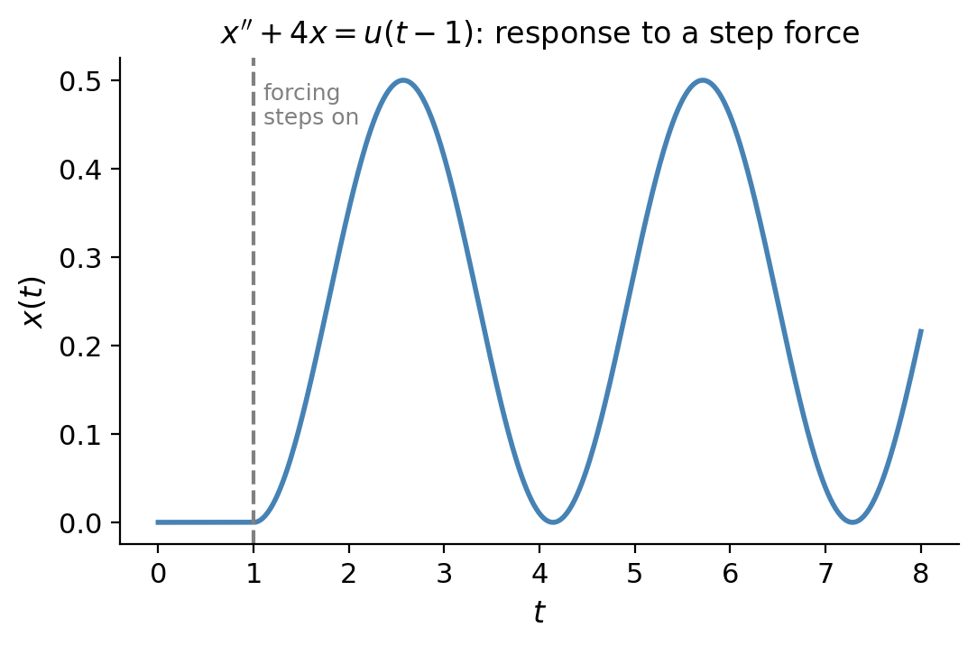
\[u_a(t) = u(t-a) = \begin{cases}0, & t < a \\ 1, & t \geq a.\end{cases}\]Its Laplace transform: \(\mathcal{L}\{u(t-a)\}=e^{-as}/s\) for \(s>0\).
Using \(u(t-a)\), any piecewise-defined function can be expressed as a single formula. For example, a rectangular pulse \(f(t)=1\) on \([a,c)\) and \(0\) otherwise equals \(f(t)=u(t-a)-u(t-c)\).
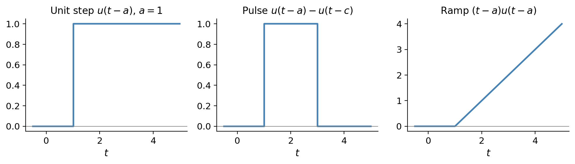
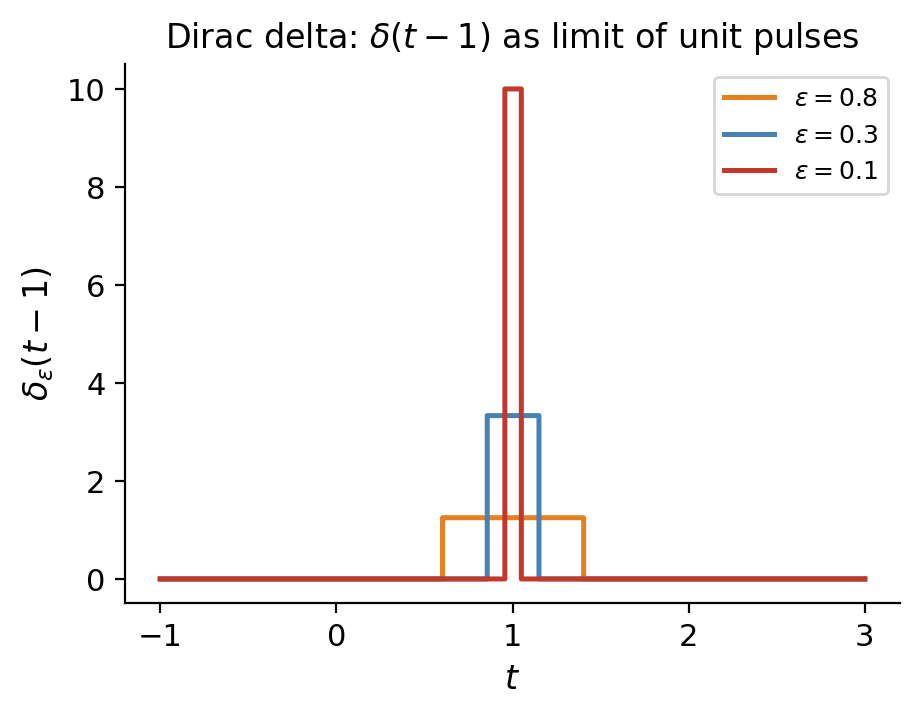
Impulsive forcing and the Dirac delta. A force applied over a very short time \(\epsilon\) with total impulse 1 can be modeled by \(f_\epsilon(t) = (1/\epsilon)\cdot\mathbf{1}_{[0,\epsilon]}(t)\). As \(\epsilon\to 0\), this becomes the Dirac delta \(\delta(t)\), characterized by \(\int_{-\infty}^\infty \delta(t)\phi(t)\,dt=\phi(0)\) for any continuous \(\phi\).
Its Laplace transform: \(\mathcal{L}\{\delta(t-a)\}=e^{-as}\) (and \(\mathcal{L}\{\delta(t)\}=1\)). Impulsive inputs localized at \(t=a\) are handled by including \(\delta(t-a)\) in the forcing term; the Laplace transform converts this to a simple exponential in \(s\).
Inverting: \(x(t)=\frac{1}{2}\sin 2t\). The hammer blow from a state of complete rest produces a sinusoidal oscillation starting immediately — as if the system had initial velocity \(x'(0^+)=1\) rather than \(0\). Physically, the impulsive force delivers momentum instantaneously: \(\int_0^{0^+}\delta(t)\,dt=1=mx'(0^+)-mx'(0^-)=1\cdot 1-0\). The delta function encodes a jump discontinuity in the derivative.
7.6 Models with Discontinuous and Impulsive Forcing
The Laplace transform truly comes into its own when the forcing function is piecewise-defined — circumstances where undetermined coefficients and variation of parameters would require solving separate ODEs on each piece and matching solutions at the discontinuities.
The forcing is \(F(t)=\cos(2t)(u(t)-u(t-2\pi))=\cos(2t)\,u(t)-\cos(2(t-2\pi))\,u(t-2\pi)\).
\[x''+4x=\cos(2t)\,u(t)-\cos(2(t-2\pi))\,u(t-2\pi), \quad x(0)=x'(0)=0.\]\[(s^2+4)X(s)=\frac{s}{s^2+4}-e^{-2\pi s}\frac{s}{s^2+4} \implies X(s)=\frac{s}{(s^2+4)^2}-e^{-2\pi s}\frac{s}{(s^2+4)^2}.\]\[x(t)=\frac{t}{4}\sin 2t-\frac{t-2\pi}{4}\sin(2(t-2\pi))\,u(t-2\pi)=\frac{t}{4}\sin 2t-\frac{t-2\pi}{4}\sin(2t)\,u(t-2\pi).\]\[x(t)=\begin{cases}\dfrac{t}{4}\sin 2t, & 0\leq t<2\pi,\\[6pt]\dfrac{\pi}{2}\sin 2t, & t\geq 2\pi.\end{cases}\]During the motor-on phase \([0,2\pi)\), this is pure resonance: the amplitude grows linearly as \(t/4\). Once the motor cuts off at \(t=2\pi\), the system settles into sinusoidal oscillation with the finite amplitude \(\pi/2\) it had at the moment of shutoff.
