AMATH 231: Calculus 4 — Vector Calculus and Fourier Series
E.R. Vrscay
Estimated study time: 1 hr 57 min
Table of contents
Chapter 1: Scalar and Vector Fields
Introduction and Motivation
This course has two major themes that together constitute the apex of the traditional calculus sequence. The first is vector calculus — the differential and integral calculus of vector-valued functions — culminating in the famous integral theorems of Green, Gauss, and Stokes. The second is Fourier analysis — the remarkable decomposition of complicated periodic functions into pure harmonics.
Vector calculus emerged historically from the study of natural phenomena: fluid flow, gravitational fields, electric and magnetic fields. These phenomena all require the concept of a field — a quantity distributed throughout space — and the vector-valued functions that model them. Fourier analysis arose from Fourier’s study of heat propagation in the early 1800s; his idea of expressing temperature distributions as infinite sums of sines and cosines launched an entire branch of analysis and remains central to signal processing, image compression (JPEG), and quantum mechanics.
Functions \( f: \mathbb{R}^n \to \mathbb{R}^m \)
The central objects of this course are functions whose inputs and outputs are both multi-dimensional. Formally, we study vector-valued functions of several variables:
\[ \mathbf{f}: \mathbb{R}^n \to \mathbb{R}^m \]The input is a point \(\mathbf{x} = (x_1, x_2, \ldots, x_n) \in \mathbb{R}^n\) and the output is a point \(\mathbf{f}(\mathbf{x}) = (f_1(\mathbf{x}), f_2(\mathbf{x}), \ldots, f_m(\mathbf{x})) \in \mathbb{R}^m\).
Notation. In these notes, vectors are written in bold, e.g., \(\mathbf{x}\), \(\mathbf{F}\). On the blackboard the arrow notation \(\vec{x}\), \(\vec{F}\) is used equivalently. The standard basis vectors of \(\mathbb{R}^3\) are \(\mathbf{i}, \mathbf{j}, \mathbf{k}\).
The domain \(D(\mathbf{f})\) is the set of points in \(\mathbb{R}^n\) at which \(\mathbf{f}\) is defined. The range \(R(\mathbf{f})\) is the set of all values assumed.
Scalar Fields
When \(m = 1\), i.e., \(f: \mathbb{R}^n \to \mathbb{R}\), we call \(f\) a scalar field (or scalar-valued function). The output is a single real number at each input point.
Examples:
- Temperature at a point in a room: \(T(x, y, z)\), a scalar field on \(\mathbb{R}^3\)
- Air pressure in the atmosphere: \(P(x, y, z, t)\), a scalar field depending on space and time
- Elevation above sea level: \(h(x, y)\), a scalar field on \(\mathbb{R}^2\)
- A greyscale photograph: \(f(x, y)\), the greyscale intensity at each point, a scalar field on a rectangular domain
Vector Fields
When \(m = n\) (or more generally \(m > 1\)), we call \(\mathbf{f}\) a vector field. At each input point \(\mathbf{x}\) in space, the field assigns an output vector. The physical interpretation is usually a velocity, force, or other directed quantity at each point.
In \(\mathbb{R}^3\), a vector field is written as
\[ \mathbf{F}(x, y, z) = F_1(x,y,z)\,\mathbf{i} + F_2(x,y,z)\,\mathbf{j} + F_3(x,y,z)\,\mathbf{k}, \]where \(F_1, F_2, F_3: \mathbb{R}^3 \to \mathbb{R}\) are the component functions.
Visualization. A vector field is visualized by drawing an arrow at each point representing the output vector. For example:
- The uniform flow field \(\mathbf{F}(x,y) = \mathbf{i}\) draws horizontal arrows everywhere — a fluid flowing rightward at constant speed.
- The radial field \(\mathbf{F}(x,y) = x\,\mathbf{i} + y\,\mathbf{j}\) draws arrows pointing outward from the origin, growing longer as we move away — a source field.
- The rotational field \(\mathbf{F}(x,y) = -y\,\mathbf{i} + x\,\mathbf{j}\) draws arrows tangent to circles around the origin — a rigid rotation. (We shall return to this field repeatedly.)
The Velocity Field of a Rotating Disc
A canonical example: a thin disc rotating counterclockwise with angular frequency \(\omega\). If \(\mathbf{r}(t) = (x(t), y(t))\) is the position of a point \(P\) on the disc, then \(x(t) = r\cos(\omega t + \theta_0)\), \(y(t) = r\sin(\omega t + \theta_0)\). Differentiating:
\[ \mathbf{v}(t) = (-\omega r \sin(\omega t + \theta_0),\; \omega r \cos(\omega t + \theta_0)) = \omega(-y\,\mathbf{i} + x\,\mathbf{j}). \]This is the rotational vector field scaled by \(\omega\). Note that \(\mathbf{v} \perp \mathbf{r}\) (since \(\mathbf{r} \cdot \mathbf{v} = 0\)), and the speed \(\|\mathbf{v}\| = \omega r\) increases with distance from the center, reflecting the fact that all points complete one rotation in the same period \(T = 2\pi/\omega\) but must traverse larger circles. The relation \(\mathbf{v} = \vec{\omega} \times \mathbf{r}\), where \(\vec{\omega} = \omega\,\mathbf{k}\), is the general formula for rigid-body rotation.
Physical Vector Fields
Gravitational Field
A mass \(M\) at the origin exerts a gravitational force on a mass \(m\) at position \(\mathbf{r} = (x,y,z)\):
\[ \mathbf{F}_{Mm}(\mathbf{r}) = -\frac{GM m}{r^3}\,\mathbf{r} = -\frac{GMm}{(x^2+y^2+z^2)^{3/2}}(x\,\mathbf{i}+y\,\mathbf{j}+z\,\mathbf{k}), \]where \(r = \|\mathbf{r}\|\) and \(G\) is Newton’s gravitational constant. The arrows point toward the origin (attractive) and diminish in length as \(r^{-2}\). The gravitational field \(\mathbf{g} = \mathbf{F}_{Mm}/m = -(GM/r^3)\mathbf{r}\) is the force per unit mass.
Electrostatic Field
A point charge \(Q\) at the origin produces an electrostatic force on charge \(q\) at \(\mathbf{r}\):
\[ \mathbf{F}(\mathbf{r}) = \frac{Qq}{4\pi\varepsilon_0 r^3}\,\mathbf{r}. \]The electric field \(\mathbf{E} = \mathbf{F}/q = Q/(4\pi\varepsilon_0 r^3)\,\mathbf{r}\) is the force per unit charge. Both the gravitational and electrostatic fields are of the special form \(\mathbf{F}(\mathbf{r}) = K\mathbf{r}/r^3\), an inverse-square central force. Such fields are conservative — they can be expressed as gradients of scalar potentials (Chapter 3).
Level Sets and Contour Plots
For a scalar field \(f: \mathbb{R}^n \to \mathbb{R}\) and a value \(C\) in its range, the \(C\)-level set is
\[ \{\mathbf{x} \in \mathbb{R}^n : f(\mathbf{x}) = C\}. \]- When \(n = 2\): level sets are usually curves (contour lines) in \(\mathbb{R}^2\), representing the intersection of the surface \(z = f(x,y)\) with the horizontal plane \(z = C\).
- When \(n = 3\): level sets are usually surfaces (level surfaces) in \(\mathbb{R}^3\).
Example. For \(f(x,y) = x^2 + y^2\), the level sets \(f = C\) are concentric circles of radius \(\sqrt{C}\) (for \(C > 0\)), the origin (for \(C = 0\)), and empty (for \(C < 0\)).
Topographic maps are physical realizations: contour lines connect points of equal elevation. The closer together the contour lines, the steeper the terrain — a relationship formalized by the gradient (Chapter 2).
Images as Scalar and Vector Fields
An important application of these ideas comes from image processing. An ideal greyscale image is a scalar field \(f: D \subset \mathbb{R}^2 \to [0,1]\), where \(f(x,y)\) represents the intensity (brightness) at pixel \((x,y)\). The value \(0\) is black, \(1\) is white, and intermediate values are shades of grey. In practice, digital images discretize both the spatial domain and the intensity range. For an 8-bit image, the domain is an \(M \times N\) integer grid and the range is \(\{0, 1, 2, \ldots, 255\}\), giving 256 grey levels.
The graph \(z = f(x,y)\) can itself be rendered as a surface plot, with grey (or colour) value indicating height. The well-known Boat test image, a \(512 \times 512\)-pixel image, illustrates this: the mast region corresponds to tall peaks in the function graph, while the sky region yields nearly flat terrain.
Colour images as vector fields. A colour image requires three numbers at each pixel — red, green, and blue intensities — so it is naturally represented by a vector-valued function:
\[ \mathbf{f}(x, y) = (r(x,y),\; g(x,y),\; b(x,y)): \mathbb{R}^2 \to \mathbb{R}^3. \]This is a vector field! The output at each pixel is a 3-vector in colour space.
Hyperspectral images. Remote-sensing instruments such as AVIRIS sample 224 wavelengths of the electromagnetic spectrum at each pixel. The result is a vector-valued function:
\[ \mathbf{f}[i,j] = (f_1[i,j], f_2[i,j], \ldots, f_M[i,j]) \in \mathbb{R}^M, \]with \(M\) up to 224. Different land-cover types (soil, vegetation, water) have distinct spectral “signatures” and can be distinguished by analysing these vectors.
Diffusion MRI (dMRI). Another powerful imaging application: diffusion MRI measures the probability that water molecules at a 3D pixel \((i,j,k)\) in the brain will diffuse in each of \(M\) directions. The result is a vector-valued function over three-dimensional space. By “following the arrows” (tracing field lines), researchers can reconstruct neural connectivity maps called connectomes — maps of the brain’s wiring.
Chapter 2: The Del Operator and Differential Operators
The Del Operator
The del operator (nabla) is the formal vector-valued differential operator
\[ \nabla = \frac{\partial}{\partial x}\,\mathbf{i} + \frac{\partial}{\partial y}\,\mathbf{j} + \frac{\partial}{\partial z}\,\mathbf{k}. \]Applied in different ways to scalar or vector fields, it generates three fundamental operators: the gradient, divergence, and curl. All three have deep geometric and physical meanings, and their interplay is the heart of vector calculus.
The Gradient
The gradient is the natural multivariable generalisation of the ordinary derivative. For a function of a single variable, \(\nabla f = f'(x)\,\mathbf{i}\).
Geometric Meaning of the Gradient
The gradient has two fundamental geometric properties:
Direction of steepest ascent. At any point \(\mathbf{x}_0\), the vector \(\nabla f(\mathbf{x}_0)\) points in the direction of most rapid increase of \(f\). Its negative, \(-\nabla f\), points in the direction of steepest descent.
Orthogonality to level sets. The gradient \(\nabla f(\mathbf{x}_0)\) is perpendicular to the level set of \(f\) passing through \(\mathbf{x}_0\). For a function of two variables, \(\nabla f\) is perpendicular to the level curve; for three variables, perpendicular to the level surface.
To see why: if \(\mathbf{r}(t)\) is any curve lying in the level surface \(f(\mathbf{x}) = C\), then \(f(\mathbf{r}(t)) = C\) for all \(t\). Differentiating using the chain rule:
\[ \frac{d}{dt}f(\mathbf{r}(t)) = \nabla f(\mathbf{r}(t)) \cdot \mathbf{r}'(t) = 0. \]Since this holds for any curve in the level surface, \(\nabla f\) is perpendicular to every tangent direction in the surface — hence perpendicular to the surface itself.
Examples
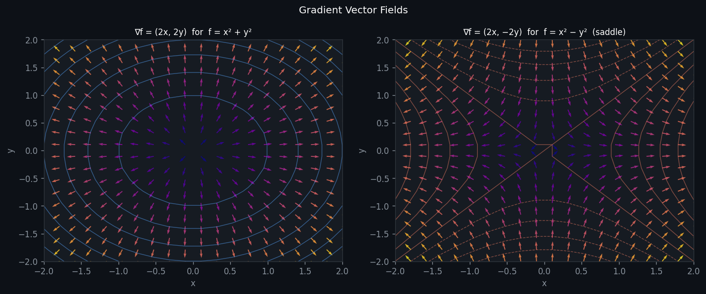
- \(f(x,y) = x^2 + y^2\): \(\nabla f = 2x\,\mathbf{i} + 2y\,\mathbf{j}\). The gradient points radially outward from the origin (perpendicular to circular level sets), and grows longer as we move away (steepness increases).
- \(T(x,y) = 50 - x^2 - 2y^2\): \(\nabla T = -2x\,\mathbf{i} - 4y\,\mathbf{j}\). Gradient points inward (toward the maximum at the origin) and has greater \(y\)-component (steeper in \(y\) due to \(-2y^2\) term).
The Directional Derivative
This is the instantaneous rate of change of \(f\) as we move from \(\mathbf{x}_0\) in direction \(\hat{\mathbf{u}}\). By the Cauchy–Schwarz inequality:
\[ |D_{\hat{u}} f| = |\nabla f \cdot \hat{\mathbf{u}}| \leq \|\nabla f\|, \]with equality when \(\hat{\mathbf{u}} = \nabla f / \|\nabla f\|\). This confirms that the gradient points in the direction of maximum rate of increase, with magnitude equal to that maximum rate.
Important Formula: \(\nabla r^n\)
For \(\mathbf{r} = x\,\mathbf{i} + y\,\mathbf{j} + z\,\mathbf{k}\) and \(r = \|\mathbf{r}\|\), one can show:
\[ \nabla r^n = n r^{n-2}\,\mathbf{r}. \]The special case \(n = -1\) gives \(\nabla(1/r) = -\mathbf{r}/r^3\), which relates directly to gravitational and electrostatic potentials (Chapter 3).
The Gradient in Image Processing: Edge Detection
A beautiful application of the gradient arises in image analysis. Let \(f(x,y)\) be the greyscale image function. At a smooth region of an image, \(f\) is nearly constant and \(\nabla f \approx \mathbf{0}\). At an edge — the boundary between two regions of different intensity — the image function undergoes a rapid change, so \(\|\nabla f\|\) is large.
For a simple step-edge, consider the function:
\[ f(x,y) = \begin{cases} 0, & -1 \leq x < 0, \\ 1, & 0 \leq x \leq 1. \end{cases} \]The gradient is zero everywhere except on the line \(x = 0\), where it is undefined (in the continuous sense), or very large in the discrete approximation. A white vertical stripe appears in the magnitude image \(\|\nabla f\|\) — precisely the edge.
For a digital image \(f[i,j]\), the discrete gradient is computed via finite differences:
\[ \nabla f[i,j] \approx \bigl(f[i+1,j] - f[i,j]\bigr)\,\mathbf{i} + \bigl(f[i,j+1] - f[i,j]\bigr)\,\mathbf{j}. \]Applied to the standard Boat test image, the magnitude \(\|\nabla f[i,j]\|\) is largest at the masts, rigging, and hull edges — the gradient is an effective edge detector. This principle underlies the Sobel, Prewitt, and Canny edge detectors used in computer vision.
The direction of the gradient, \(\theta = \arctan(\partial f/\partial y, \partial f/\partial x)\), indicates the angle at which the edge runs, providing additional information for image segmentation.
Divergence
The divergence is obtained by applying the del operator as a dot product with \(\mathbf{F}\).
Physical Meaning: Source/Sink Density
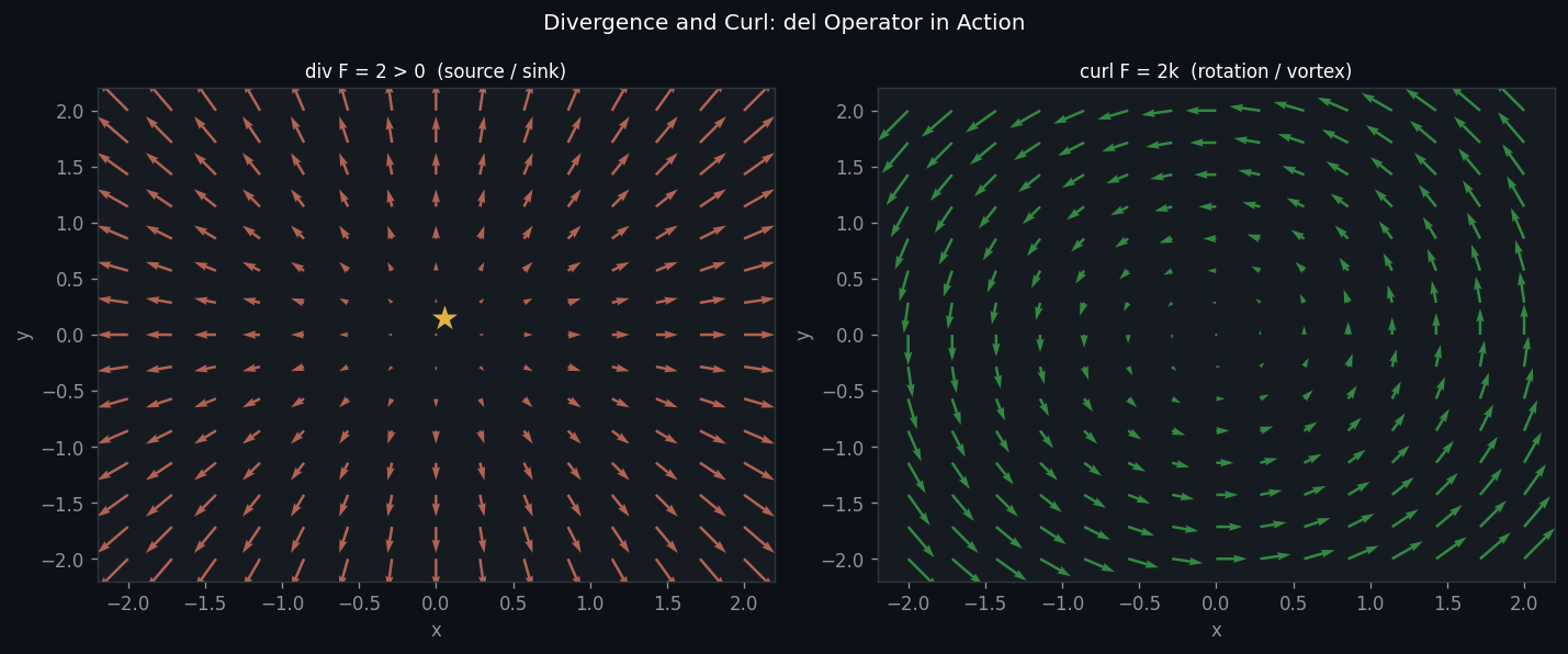
The divergence measures the “net outward flow per unit volume” at a point — equivalently, the density of sources (positive divergence) or sinks (negative divergence) in a vector field.
Intuition. Imagine a fluid with velocity field \(\mathbf{v}(\mathbf{x})\). If \(\nabla \cdot \mathbf{v} > 0\) at a point, more fluid is flowing out of a small region around that point than flowing in — there is a source. If \(\nabla \cdot \mathbf{v} < 0\), there is a sink. If \(\nabla \cdot \mathbf{v} = 0\) everywhere, the fluid is incompressible (volume-preserving), as is the case for most liquids.
This physical interpretation is made precise by Gauss’s Divergence Theorem (Chapter 8):
\[ \nabla \cdot \mathbf{F}(\mathbf{p}) = \lim_{\varepsilon \to 0} \frac{1}{V(D_\varepsilon)} \iint_{S_\varepsilon} \mathbf{F} \cdot \hat{\mathbf{n}}\, dS, \]where \(S_\varepsilon\) is a small sphere of radius \(\varepsilon\) centred at \(\mathbf{p}\) and \(V(D_\varepsilon) = \frac{4}{3}\pi\varepsilon^3\) is its volume.
Examples
- \(\mathbf{F} = x\,\mathbf{i} + y\,\mathbf{j} + z\,\mathbf{k}\): \(\nabla \cdot \mathbf{F} = 3\). Constant positive divergence — every point is a source; the field flows radially outward everywhere.
- \(\mathbf{F} = -y\,\mathbf{i} + x\,\mathbf{j}\): \(\nabla \cdot \mathbf{F} = 0\). Pure rotation; no sources or sinks.
- \(\mathbf{F} = \mathbf{r}/r^3\) (gravitational/electrostatic field): \(\nabla \cdot \mathbf{F} = 0\) for \(\mathbf{r} \neq \mathbf{0}\) — no sources away from the origin.
Curl
For a planar vector field \(\mathbf{F}(x,y) = F_1\mathbf{i} + F_2\mathbf{j}\) (setting \(F_3 = 0\) and assuming no \(z\)-dependence):
\[ \nabla \times \mathbf{F} = \left(\frac{\partial F_2}{\partial x} - \frac{\partial F_1}{\partial y}\right)\mathbf{k}, \]which points in the \(\mathbf{k}\) direction only.
Physical Meaning: Rotation/Vorticity
The curl measures the local infinitesimal rotation in a vector field. In fluid mechanics, if \(\mathbf{v}\) is a velocity field, the quantity
\[ \Omega(x,y) = \left[\nabla \times \mathbf{v}\right]_z = \frac{\partial v_2}{\partial x} - \frac{\partial v_1}{\partial y} \]is called the vorticity of the fluid at \((x,y)\). A non-zero vorticity at a point means a small “paddle wheel” placed there would be set spinning by the fluid.
The precise interpretation: using Green’s Theorem on a small disc \(D_\varepsilon\) of radius \(\varepsilon\),
\[ \oint_{C_\varepsilon} \mathbf{F} \cdot d\mathbf{x} = \iint_{D_\varepsilon} \Omega(x,y)\, dA \approx \Omega(\mathbf{p})\cdot \pi\varepsilon^2, \]so
\[ \Omega(\mathbf{p}) = \lim_{\varepsilon \to 0} \frac{1}{\pi\varepsilon^2} \oint_{C_\varepsilon} \mathbf{F} \cdot d\mathbf{x}. \]The curl is the circulation per unit area.
Examples
- \(\mathbf{F} = -y\,\mathbf{i} + x\,\mathbf{j}\) (rotating disc, \(\omega = 1\)): \(\nabla \times \mathbf{F} = 2\mathbf{k}\). Constant non-zero curl everywhere — the field is uniformly rotational.
- \(\mathbf{F} = x\,\mathbf{i} + y\,\mathbf{j}\): \(\nabla \times \mathbf{F} = \mathbf{0}\). Source field; no rotation.
- \(\mathbf{F} = \mathbf{r}/r^3\): \(\nabla \times \mathbf{F} = \mathbf{0}\) for \(\mathbf{r} \neq \mathbf{0}\). Central force fields are irrotational away from the origin.
The Laplacian
The Laplacian is the scalar result of taking the divergence of the gradient. It measures how much the value of \(f\) at a point differs from the average of \(f\) in a surrounding neighbourhood (a fact made precise via the mean-value property). Functions satisfying \(\nabla^2 f = 0\) are called harmonic; they appear naturally as steady-state solutions to the heat and wave equations.
Key Identities
Two fundamental identities constrain the gradient, divergence, and curl:
Both identities follow from the equality of mixed partial derivatives (Clairaut’s theorem). They have profound consequences: the first means that gradient fields are irrotational (zero curl), which is the test for conservatism; the second means that curl fields are solenoidal (zero divergence), which underpins the vector potential in electromagnetism.
Chapter 3: Conservative Vector Fields and Potential Functions
Conservative Forces in One Dimension
Before treating the general case, consider a mass \(m\) moving along the \(x\)-axis under a force \(F(x)\). Newton’s law gives \(F = ma = mx''(t)\). The potential energy associated with the force is defined as
\[ V(x) = -\int_{x_0}^{x} F(s)\, ds, \]where \(x_0\) is a reference point. By the Fundamental Theorem of Calculus:
\[ V'(x) = -F(x), \quad \text{equivalently,} \quad F(x) = -V'(x). \]A force that can be written as \(F = -V'\) is called conservative. The total mechanical energy is
\[ E(t) = \frac{1}{2}mv(t)^2 + V(x(t)). \]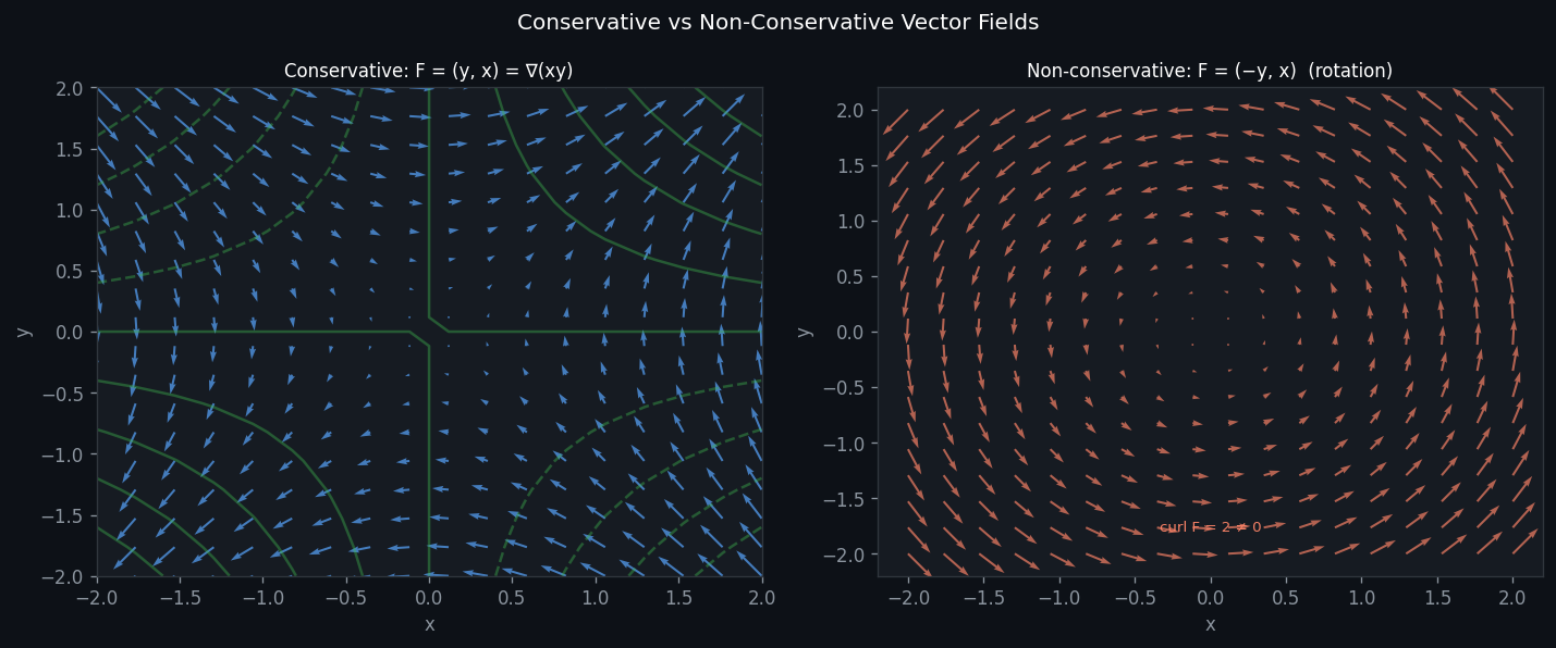
Conservative Forces in Higher Dimensions
- a gradient field if there exists a scalar function \(f: \mathbb{R}^n \to \mathbb{R}\) such that \(\mathbf{F} = \nabla f\);
- a conservative force (physics convention) if \(\mathbf{F} = -\nabla V\) for some potential energy \(V\).
Test for Conservatism
How do we determine whether a given vector field \(\mathbf{F}\) is conservative? The answer is provided by the curl:
The conditions \(\nabla \times \mathbf{F} = \mathbf{0}\) expand to three scalar equations:
\[ \frac{\partial F_1}{\partial y} = \frac{\partial F_2}{\partial x}, \quad \frac{\partial F_1}{\partial z} = \frac{\partial F_3}{\partial x}, \quad \frac{\partial F_2}{\partial z} = \frac{\partial F_3}{\partial y}. \]For a planar field \(\mathbf{F}(x,y) = F_1\mathbf{i} + F_2\mathbf{j}\), only the first condition is needed: \(\partial F_2/\partial x = \partial F_1/\partial y\).
Important caveat. The domain must be simply connected (every loop can be contracted to a point without leaving the domain). The field \(\mathbf{F} = (-y\,\mathbf{i} + x\,\mathbf{j})/(x^2 + y^2)\), defined on \(\mathbb{R}^2 \setminus \{0\}\) (not simply connected), satisfies \(\nabla \times \mathbf{F} = \mathbf{0}\) but is not conservative — the line integral around any loop enclosing the origin equals \(2\pi \neq 0\).
Finding the Potential Function
Given that \(\mathbf{F} = \nabla f\), i.e.,
\[ \frac{\partial f}{\partial x} = F_1, \quad \frac{\partial f}{\partial y} = F_2, \quad \frac{\partial f}{\partial z} = F_3, \]we find \(f\) by partial antidifferentiation: integrate \(F_1\) with respect to \(x\) (treating \(y,z\) as constants) to get a candidate for \(f\), then differentiate with respect to \(y\) and match with \(F_2\) to pin down the “constant” of integration (which may depend on \(y,z\)), and so on.
Physical Examples of Conservative Fields
Gravitational Potential
The gravitational force \(\mathbf{F} = -GMm\mathbf{r}/r^3\) is conservative. Using \(\nabla(1/r) = -\mathbf{r}/r^3\):
\[ \mathbf{F} = -\nabla V, \quad V(r) = -\frac{GMm}{r}. \]The gravitational potential energy decreases to \(-\infty\) as \(r \to 0\) and approaches \(0\) as \(r \to \infty\). Two masses bound together (like the Earth-Moon system) have negative total energy.
Electrostatic Potential
The electrostatic force \(\mathbf{F} = Qq/(4\pi\varepsilon_0 r^3)\,\mathbf{r}\) is conservative with potential energy
\[ V(r) = \frac{Qq}{4\pi\varepsilon_0 r}, \quad \text{and electrostatic potential } \Phi(r) = \frac{Q}{4\pi\varepsilon_0 r}. \]The level sets of \(\Phi\) are spheres centred at the origin; the electric field \(\mathbf{E} = -\nabla\Phi\) points radially (outward for \(Q > 0\)) and is perpendicular to these equipotential surfaces.
Chapter 4: Line Integrals
Arc Length
Before integrating vector fields along curves, we recall the arc length integral. A curve \(C\) parametrized by \(\mathbf{g}(t) = (x(t), y(t), z(t))\), \(t \in [a,b]\), has arc length
\[ L = \int_C ds = \int_a^b \|\mathbf{g}'(t)\|\, dt. \]The element \(ds = \|\mathbf{g}'(t)\| dt\) is the “speed” \(\times\) \(dt\). The integral of a scalar function \(f\) over \(C\) is
\[ \int_C f\, ds = \int_a^b f(\mathbf{g}(t))\,\|\mathbf{g}'(t)\|\, dt. \]If \(f = 1\) this recovers arc length; if \(f\) is a linear mass density, the integral gives total mass.
Line Integrals of Vector Fields
The physically central integral is the work integral (line integral of a vector field):
Physical motivation. If a force \(\mathbf{F}(\mathbf{x})\) acts on a mass moving from \(P\) to \(Q\) along \(C\), the work done is exactly this integral. The dot product \(\mathbf{F} \cdot \mathbf{g}' dt\) picks out the component of force along the direction of motion.
Computation Procedure
- Parametrize \(C\): \(\mathbf{x}(t) = \mathbf{g}(t)\), \(t \in [a,b]\), with \(\mathbf{g}(a) = P\), \(\mathbf{g}(b) = Q\).
- Compute \(\mathbf{g}'(t)\).
- Evaluate \(\mathbf{F}(\mathbf{g}(t))\).
- Form the dot product \(\mathbf{F}(\mathbf{g}(t)) \cdot \mathbf{g}'(t)\) and integrate over \([a,b]\).
\(\mathbf{g}'(t) = (-\sin t, \cos t, 1)\). \(\mathbf{F}(\mathbf{g}(t)) = (2\cos t, 4\sin t, t)\). Dot product: \(-2\cos t\sin t + 4\sin t\cos t + t = 2\sin t\cos t + t\). Integral:
\[ \int_0^{2\pi}(2\sin t\cos t + t)\, dt = \left[\sin^2 t + \frac{t^2}{2}\right]_0^{2\pi} = 0 + 2\pi^2 = 2\pi^2. \]The same value is obtained along any path from \((1,0,0)\) to \((1,0,2\pi)\), since \(\mathbf{F} = \nabla f\) with \(f = x^2 + 2y^2 + \frac{1}{2}z^2\) (verified: this is a gradient field).
Properties
Orientation. Reversing the direction of traversal negates the integral: \(\int_{C_{QP}} \mathbf{F} \cdot d\mathbf{x} = -\int_{C_{PQ}} \mathbf{F} \cdot d\mathbf{x}\). (Proof: reparametrize with \(\tau = a + b - t\).)
Linearity. \(\int_C (c\mathbf{F} + \mathbf{G}) \cdot d\mathbf{x} = c\int_C \mathbf{F} \cdot d\mathbf{x} + \int_C \mathbf{G} \cdot d\mathbf{x}\).
Additivity. If \(C = C_1 \cup C_2\) (consistent orientation): \(\int_C = \int_{C_1} + \int_{C_2}\).
Parametrization independence. The value of \(\int_C \mathbf{F} \cdot d\mathbf{x}\) does not depend on which parametrization of \(C\) is used (only on the curve and its orientation).
The Fundamental Theorem for Line Integrals
This is the most important theorem for line integrals, generalising the Fundamental Theorem of Calculus to higher dimensions.
Therefore:
\[ \int_C \nabla f \cdot d\mathbf{x} = \int_{t_1}^{t_2} \nabla f(\mathbf{g}(t)) \cdot \mathbf{g}'(t)\, dt = \int_{t_1}^{t_2} \frac{d}{dt}f(\mathbf{g}(t))\, dt = f(\mathbf{g}(t_2)) - f(\mathbf{g}(t_1)) = f(\mathbf{x}_2) - f(\mathbf{x}_1). \]The connection to FTC II is clear: \(\int_a^b f'(x)\, dx = f(b) - f(a)\) is exactly this theorem for \(n = 1\), since \(\nabla f = f'\mathbf{i}\).
Consequences for Conservative Forces
If a conservative force \(\mathbf{F} = -\nabla V\) moves a mass from \(A\) to \(B\), the work done is:
\[ W = \int_{C_{AB}} \mathbf{F} \cdot d\mathbf{x} = -[V(B) - V(A)] = V(A) - V(B) = -\Delta V. \]By conservation of energy, \(V(A) - V(B) = K(B) - K(A)\), so \(W = \Delta K\): the work-energy theorem. The work done by a conservative force equals the change in kinetic energy. Moreover, if the mass returns to \(A\) (closed path), then \(W = V(A) - V(A) = 0\): no net work over any closed path — this is the hallmark of a conservative force.
Chapter 5: Green’s Theorem
Statement
Green’s Theorem relates a line integral around a closed curve to a double integral over the enclosed region. It is the two-dimensional version of Stokes’ Theorem and one of the great theorems of calculus.
The left side is the circulation of \(\mathbf{F}\) around \(C\); the right side is the integral of the curl’s \(z\)-component over \(D\).
There is an equivalent flux/divergence form: with \(\hat{\mathbf{n}}\) the outward unit normal to \(C\) and \(\mathbf{F} = F_1\mathbf{i} + F_2\mathbf{j}\),
\[ \oint_C \mathbf{F} \cdot \hat{\mathbf{n}}\, ds = \iint_D \left(\frac{\partial F_1}{\partial x} + \frac{\partial F_2}{\partial y}\right) dA = \iint_D \nabla \cdot \mathbf{F}\, dA. \]These are the circulation form and flux form of Green’s Theorem, respectively.
Proof Sketch
We prove the theorem for a rectangle \(D = [a,b] \times [c,d]\), then extend by approximation.
For the rectangle, the boundary \(C\) consists of four sides. The circulation integral splits as:
\[ \oint_C F_1\, dx + F_2\, dy = \left(\int_{\text{bottom}} + \int_{\text{right}} + \int_{\text{top}} + \int_{\text{left}}\right)(F_1\, dx + F_2\, dy). \]Consider only the \(F_1\, dx\) parts (the \(F_2\, dy\) parts are analogous). On the bottom edge (\(y = c\), \(x\): \(a \to b\)):
\[ \int_a^b F_1(x,c)\, dx. \]On the top edge (\(y = d\), \(x\): \(b \to a\)):
\[ -\int_a^b F_1(x,d)\, dx. \]Sum: \(\int_a^b [F_1(x,c) - F_1(x,d)]\, dx = -\int_a^b \int_c^d \frac{\partial F_1}{\partial y}\, dy\, dx\). Similarly for \(F_2\, dy\). Adding both contributions yields the result.
For a general region, approximate \(D\) by a grid of small rectangles. Interior edges cancel (each is shared by two rectangles traversed in opposite orientations), leaving only the outer boundary.
Curl Form Rewritten
Since \(\partial F_2/\partial x - \partial F_1/\partial y = (\nabla \times \mathbf{F})_z\), Green’s theorem reads:
\[ \oint_C \mathbf{F} \cdot d\mathbf{x} = \iint_D (\nabla \times \mathbf{F})_z\, dA. \]This is the 2D precursor of Stokes’ Theorem: the circulation around the boundary equals the integrated vorticity over the interior. The \(z\)-component arises because \(\hat{\mathbf{k}}\) is the outward unit normal to the flat region \(D\) in \(\mathbb{R}^3\).
Applications
Area of a Region
Setting \(\mathbf{F} = (0, x)\) (so \(\partial F_2/\partial x - \partial F_1/\partial y = 1\)):
\[ \text{Area}(D) = \oint_C x\, dy. \]Or with \(\mathbf{F} = (-y, 0)\): Area \(= -\oint_C y\, dx\). The symmetric average gives the surveyor’s formula:
\[ \text{Area}(D) = \frac{1}{2}\oint_C (x\, dy - y\, dx). \]Connecting Conservatism and Path Independence
From Green’s theorem: if \(\nabla \times \mathbf{F} = \mathbf{0}\) on a simply-connected region \(D\), then for any closed curve \(C\) in \(D\):
\[ \oint_C \mathbf{F} \cdot d\mathbf{x} = \iint_D 0\, dA = 0. \]A vector field has zero circulation around every closed loop if and only if it is path-independent (conservative).
Physical Curl Interpretation
The curl gives the local rotation density of the field. Green’s theorem says: summing this local rotation over all of \(D\) gives the total circulation around the boundary. Positive curl means counterclockwise local rotation; negative means clockwise. A field with zero curl everywhere has zero net circulation around any boundary — it is irrotational.
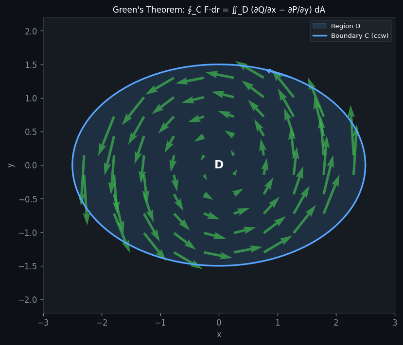
Here \(F_1 = -y\), \(F_2 = x\), so \(\partial F_2/\partial x - \partial F_1/\partial y = 1 + 1 = 2\). By Green’s Theorem:
\[ \oint_C (-y\,dx + x\,dy) = \iint_{x^2+y^2\leq 1} 2\, dA = 2\pi. \]Direct verification: parametrize as \((cos t, \sin t)\), \(t \in [0, 2\pi]\): integrand \(= \sin^2 t + \cos^2 t = 1\), integral \(= 2\pi\). Consistent.
Chapter 6: Curl of a Vector Field
Definition and Calculation
The curl was defined in Chapter 2 using the del operator. Here we develop its properties more fully.
For \(\mathbf{F} = F_1\mathbf{i} + F_2\mathbf{j} + F_3\mathbf{k}\):
\[ \nabla \times \mathbf{F} = \left(\frac{\partial F_3}{\partial y} - \frac{\partial F_2}{\partial z}\right)\mathbf{i} + \left(\frac{\partial F_1}{\partial z} - \frac{\partial F_3}{\partial x}\right)\mathbf{j} + \left(\frac{\partial F_2}{\partial x} - \frac{\partial F_1}{\partial y}\right)\mathbf{k}. \]The three components measure rotation about the three coordinate axes:
- \((\nabla \times \mathbf{F})_x\): rotation about the \(x\)-axis (vorticity in the \(yz\)-plane)
- \((\nabla \times \mathbf{F})_y\): rotation about the \(y\)-axis (vorticity in the \(xz\)-plane)
- \((\nabla \times \mathbf{F})_z\): rotation about the \(z\)-axis (vorticity in the \(xy\)-plane)
Properties
This means: gradient fields (conservative fields) are irrotational. Equivalently, if you can measure that a field has zero curl everywhere on a simply-connected domain, it is conservative and has a potential.
This means: every curl field is solenoidal (divergence-free). In electromagnetism, the magnetic field \(\mathbf{B} = \nabla \times \mathbf{A}\) (where \(\mathbf{A}\) is the vector potential) automatically satisfies \(\nabla \cdot \mathbf{B} = 0\) — one of Maxwell’s equations.
Vorticity and Physical Interpretation
In fluid mechanics, the vorticity vector \(\boldsymbol{\Omega} = \nabla \times \mathbf{v}\) at a point describes the local angular velocity of the fluid. Specifically, the angular velocity of the fluid at a point (as measured by a tiny tracer paddle wheel) is \(\boldsymbol{\Omega}/2\).
For rigid-body rotation \(\mathbf{v} = \omega(-y\mathbf{i} + x\mathbf{j})\): \(\nabla \times \mathbf{v} = 2\omega\mathbf{k}\). The vorticity is uniform, and the angular velocity of any fluid element is \(\omega\mathbf{k}\) — consistent with uniform rotation.
For a velocity field that resembles rotation but is not rigid (e.g., the potential vortex \(\mathbf{v} = (-y, x)/(x^2+y^2)\)), the vorticity is zero everywhere except the origin. This reflects that individual fluid particles travel on circles but do not rotate about their own axes — a distinction invisible without the curl.
Chapter 7: Surface Integrals
Parametrized Surfaces
A parametrized surface \(S\) is described by a function
\[ \mathbf{g}(u,v) = (x(u,v),\, y(u,v),\, z(u,v)), \quad (u,v) \in D \subset \mathbb{R}^2. \]The domain \(D\) in parameter space maps to the surface \(S\) in \(\mathbb{R}^3\).
Standard examples:
- \[ \mathbf{g}(u,v) = (R\cos u\sin v,\; R\sin u\sin v,\; R\cos v). \]
Cylinder \(x^2 + y^2 = a^2\), \(0 \leq z \leq b\): use \(\mathbf{g}(u,v) = (a\cos u, a\sin u, v)\), \(u \in [0,2\pi]\), \(v \in [0,b]\).
Graph \(z = f(x,y)\) over region \(D_{xy}\): use \(\mathbf{g}(u,v) = (u, v, f(u,v))\).
Tangent Vectors and Normal Vector
Two curves lie in the surface through each point \(\mathbf{g}(u_0, v_0)\):
- Fix \(v = v_0\), vary \(u\): tangent vector \(\mathbf{T}_u = \partial\mathbf{g}/\partial u\).
- Fix \(u = u_0\), vary \(v\): tangent vector \(\mathbf{T}_v = \partial\mathbf{g}/\partial v\).
The normal vector to \(S\) at \(\mathbf{g}(u_0, v_0)\) is:
\[ \mathbf{N}(u,v) = \mathbf{T}_u \times \mathbf{T}_v = \frac{\partial\mathbf{g}}{\partial u} \times \frac{\partial\mathbf{g}}{\partial v}. \]The choice of sign (plus or minus) determines the orientation of the surface. By convention, for a closed surface (like a sphere), the outward normal is chosen.
The surface area element is:
\[ dS = \|\mathbf{N}(u,v)\|\, du\, dv. \]Sphere example. For the sphere of radius \(R\):
\[ \mathbf{T}_u \times \mathbf{T}_v = -R^2 \sin v\,\mathbf{g}(u,v)/R = -R\sin v\,\hat{\mathbf{r}}, \]so \(\|\mathbf{N}\| = R^2\sin v\) — the familiar Jacobian from spherical coordinates. The area element is \(dS = R^2 \sin v\, du\, dv\), and:
\[ \text{Area}(S_R) = \int_0^{2\pi}\int_0^{\pi} R^2\sin v\, dv\, du = 4\pi R^2. \]Scalar Surface Integrals
Interpretations:
- \(f = 1\): area of \(S\).
- \(f = \) mass density (per unit area): total mass of a thin shell.
- \(f = \) charge density: total charge on a surface.
Flux Integrals (Vector Surface Integrals)
The most physically important surface integral computes the flux of a vector field through a surface.
Physical meaning. If \(\mathbf{F} = \rho\mathbf{v}\) is the mass flux density of a fluid (mass per unit time per unit area), then \(\iint_S \mathbf{F} \cdot \hat{\mathbf{n}}\, dS\) is the total mass of fluid crossing \(S\) per unit time.
Special case: graph \(z = g(x,y)\). For a surface given as a graph, with the upward orientation:
\[ \mathbf{N} = (-g_x, -g_y, 1), \]so the flux integral becomes:
\[ \iint_S \mathbf{F} \cdot d\mathbf{S} = \iint_{D_{xy}} \bigl(-F_1 g_x - F_2 g_y + F_3\bigr)\, dA. \]On the sphere, \(\hat{\mathbf{n}} = \mathbf{g}/R\) (radially outward). Then \(\mathbf{F} \cdot \hat{\mathbf{n}} = (1/R^3)\mathbf{r} \cdot (\mathbf{r}/R) = R^2/R^4 = 1/R^2\). Flux \(= (1/R^2)\cdot 4\pi R^2 = 4\pi\). This equals \(4\pi\) regardless of \(R\) — a consequence of Gauss’s Divergence Theorem.
Chapter 8: Gauss’s Divergence Theorem
Statement
The theorem equates the total outward flux through the surface with the integrated source density throughout the volume. It is the three-dimensional generalisation of Green’s flux/divergence form.
Proof Sketch
We prove it for a box \(V = [a_1, b_1] \times [a_2, b_2] \times [a_3, b_3]\). Consider the \(F_3\) contribution. The top face (\(z = b_3\), normal \(+\mathbf{k}\)) and bottom face (\(z = a_3\), normal \(-\mathbf{k}\)) contribute:
\[ \iint_{\text{top}} F_3\, dA - \iint_{\text{bottom}} F_3\, dA = \iint_{[a_1,b_1]\times[a_2,b_2]} [F_3(x,y,b_3) - F_3(x,y,a_3)]\, dA. \]By the Fundamental Theorem of Calculus in \(z\):
\[ = \iiint_V \frac{\partial F_3}{\partial z}\, dV. \]Doing the same for \(F_1\) (left/right faces) and \(F_2\) (front/back faces) and adding gives the full divergence theorem for the box. General regions are handled by approximating with a grid of boxes — interior face contributions cancel, leaving the outer boundary.
Physical Interpretation: Divergence as Local Source Density
Using the mean value theorem for integrals: shrink a sphere \(S_\varepsilon\) of radius \(\varepsilon\) about a point \(\mathbf{p}\) to zero:
\[ \iint_{S_\varepsilon} \mathbf{F} \cdot \hat{\mathbf{n}}\, dS = \nabla \cdot \mathbf{F}(\mathbf{q}_\varepsilon) \cdot V(D_\varepsilon), \]where \(\mathbf{q}_\varepsilon \in D_\varepsilon\). Dividing by \(V(D_\varepsilon) = \frac{4}{3}\pi\varepsilon^3\) and taking \(\varepsilon \to 0\):
\[ \nabla \cdot \mathbf{F}(\mathbf{p}) = \lim_{\varepsilon \to 0} \frac{\text{total outward flux through } S_\varepsilon}{V(D_\varepsilon)}. \]The divergence is the outward flux per unit volume at a point — the density of sources (positive) or sinks (negative).
Conservation Laws and the Continuity Equation
The Divergence Theorem is the key to deriving conservation laws in mathematical physics. Let \(u(\mathbf{x}, t)\) be the concentration (amount per unit volume) of some substance \(X\) — it could be a chemical solute, the density of a gas, or heat energy. Let \(\mathbf{j}(\mathbf{x},t)\) be the flux density vector: the rate per unit area at which \(X\) crosses a surface element at \(\mathbf{x}\).
For any fixed region \(D\) with boundary \(\partial D\), the total amount of \(X\) in \(D\) is
\[ U(t) = \iiint_D u(\mathbf{x},t)\, dV. \]By Leibniz’s rule (differentiating under the integral):
\[ U'(t) = \iiint_D \frac{\partial u}{\partial t}\, dV. \]The only way \(U\) can change (assuming no creation or destruction of \(X\) within \(D\)) is by flux through the boundary:
\[ U'(t) = -\iint_{\partial D} \mathbf{j} \cdot \hat{\mathbf{n}}\, dS. \]The minus sign: outward flux decreases the amount inside. By the Divergence Theorem:
\[ -\iint_{\partial D} \mathbf{j} \cdot \hat{\mathbf{n}}\, dS = -\iiint_D \nabla \cdot \mathbf{j}\, dV. \]Therefore:
\[ \iiint_D \left(\frac{\partial u}{\partial t} + \nabla \cdot \mathbf{j}\right) dV = 0. \]Since this holds for every region \(D\), and the integrand is continuous, the du Bois-Reymond Lemma (multi-dimensional version: if \(\int_D f\, dV = 0\) for all \(D\) and \(f\) is continuous, then \(f \equiv 0\)) gives the continuity equation:
\[ \frac{\partial u}{\partial t} + \nabla \cdot \mathbf{j} = 0. \]This single equation encodes conservation of \(X\).
The Diffusion and Heat Equations
Applying the continuity equation to specific physical scenarios:
Diffusion (Fick’s Law)
For a chemical solute diffusing in a solvent, experimental evidence (Fick’s law of diffusion) shows that the flux flows from high to low concentration:
\[ \mathbf{j} = -\kappa\, \nabla u, \]where \(\kappa > 0\) is the diffusivity. Substituting into the continuity equation:
\[ \frac{\partial u}{\partial t} = \nabla \cdot (\kappa\, \nabla u) = \kappa\, \nabla^2 u. \]This is the diffusion equation: \(\partial u/\partial t = \kappa\, \nabla^2 u\).
Heat Conduction (Fourier’s Law)
For heat in a conducting medium, let \(T(\mathbf{x},t)\) be temperature. The heat energy density is \(u = c\rho T\) (where \(c\) is specific heat and \(\rho\) is density). The heat flux is (Fourier’s law of heat conduction):
\[ \mathbf{j} = -k\, \nabla T. \]Substituting:
\[ c\rho\, \frac{\partial T}{\partial t} = \nabla \cdot (k\, \nabla T) = k\, \nabla^2 T. \]Setting \(\kappa = k/(c\rho)\) (thermal diffusivity):
\[ \boxed{\frac{\partial T}{\partial t} = \kappa\, \nabla^2 T.} \]This is the heat equation — the PDE for which Fourier originally developed his series (Chapter 12).
Physical meaning. The Laplacian \(\nabla^2 T\) measures how much \(T\) at a point differs from the average of \(T\) in its neighbourhood. Where \(T\) is above average (\(\nabla^2 T < 0\)), the temperature decreases; where below average, it increases. The system evolves toward a uniform temperature: equilibrium.
Incompressible Fluid (Continuity)
For a fluid with density \(\rho(\mathbf{x},t)\) and velocity \(\mathbf{v}\), setting \(\mathbf{j} = \rho\mathbf{v}\) and \(u = \rho\):
\[ \frac{\partial\rho}{\partial t} + \nabla \cdot (\rho\mathbf{v}) = 0. \]For an incompressible fluid (\(\rho = \rho_0 = \text{const}\)), this reduces to \(\nabla \cdot \mathbf{v} = 0\): the velocity field is divergence-free (solenoidal).
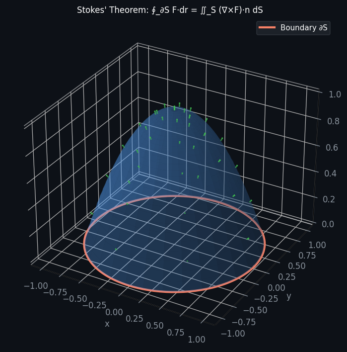
Chapter 9: Stokes’ Theorem
Statement
Stokes’ Theorem generalises Green’s Theorem to surfaces in three dimensions: it relates the circulation of a vector field around a closed curve to the flux of the curl through any surface bounded by that curve.
Orientation convention. The positive orientation of \(C\) relative to \(S\): if you walk along \(C\) with your head pointing in the direction of \(\hat{\mathbf{n}}\), the surface \(S\) should be on your left. Equivalently, curl the fingers of the right hand in the direction of traversal of \(C\); the thumb points in the direction of \(\hat{\mathbf{n}}\).
Green’s Theorem as a Special Case
When \(S\) is a flat region \(D\) in the \(xy\)-plane with outward normal \(\hat{\mathbf{n}} = \mathbf{k}\):
\[ \iint_D (\nabla \times \mathbf{F}) \cdot \mathbf{k}\, dA = \iint_D \left(\frac{\partial F_2}{\partial x} - \frac{\partial F_1}{\partial y}\right) dA = \oint_C \mathbf{F} \cdot d\mathbf{x}. \]This is Green’s Theorem. Stokes’ Theorem thus subsumes Green’s Theorem as the special case where the surface is a plane.
Proof Sketch
Approximate \(S\) by a mesh of small surface patches. Apply Green’s Theorem to each patch (projected locally onto its tangent plane). Adjacent patches share boundaries in opposite orientations, so interior contributions cancel, leaving only the outer boundary \(C = \partial S\).
More carefully: parametrize \(S\) by \(\mathbf{g}(u,v)\), \((u,v) \in D\). By Green’s theorem applied in the \((u,v)\) plane to the vector field \(\mathbf{G}(u,v) = \mathbf{F}(\mathbf{g}(u,v)) \cdot \partial\mathbf{g}/\partial u\) and \(\mathbf{H}(u,v) = \mathbf{F}(\mathbf{g}(u,v)) \cdot \partial\mathbf{g}/\partial v\), the equality can be established after careful chain-rule manipulation.
Applications
Computing Circulation via Stokes
Stokes’ theorem is most useful when computing the line integral \(\oint_C \mathbf{F} \cdot d\mathbf{x}\) directly is difficult, but when \(\nabla \times \mathbf{F}\) is simple.
\(\nabla \times \mathbf{F} = 2\mathbf{k}\). By Stokes:
\[ \oint_C \mathbf{F} \cdot d\mathbf{x} = \iint_S 2\mathbf{k} \cdot \mathbf{k}\, dA = 2\cdot\pi(1)^2 = 2\pi. \]Simplifying via Surface Independence
A profound consequence of Stokes’ Theorem: the integral \(\iint_S (\nabla \times \mathbf{F}) \cdot d\mathbf{S}\) depends only on the boundary \(\partial S = C\), not on which surface \(S\) spanning \(C\) you choose. This is because if \(S_1\) and \(S_2\) both span \(C\), then \(S_1 - S_2\) forms a closed surface and by the divergence theorem:
\[ \iint_{S_1} (\nabla \times \mathbf{F}) \cdot d\mathbf{S} - \iint_{S_2} (\nabla \times \mathbf{F}) \cdot d\mathbf{S} = \iiint_V \nabla \cdot (\nabla \times \mathbf{F})\, dV = 0, \]since \(\nabla \cdot (\nabla \times \mathbf{F}) = 0\) always.
Zero Curl and Conservative Fields
For a field with \(\nabla \times \mathbf{F} = \mathbf{0}\) on a simply-connected domain:
\[ \oint_C \mathbf{F} \cdot d\mathbf{x} = \iint_S \mathbf{0} \cdot d\mathbf{S} = 0 \]for every closed curve \(C\). This confirms that zero-curl fields are conservative (path-independent) on simply-connected domains.
The Hierarchy of Integral Theorems
The three great theorems have a common structure: they relate an integral over a domain to an integral over its boundary.
| Theorem | Domain | Boundary | Operator |
|---|---|---|---|
| FTC | \([a,b]\) | \(\{a, b\}\) | derivative |
| Green | region \(D \subset \mathbb{R}^2\) | curve \(C = \partial D\) | curl (\(z\)-component) |
| Stokes | surface \(S \subset \mathbb{R}^3\) | curve \(C = \partial S\) | curl |
| Gauss | volume \(V \subset \mathbb{R}^3\) | surface \(S = \partial V\) | divergence |
All are manifestations of the same abstract theorem in differential geometry: \(\int_\Omega d\omega = \int_{\partial\Omega} \omega\), where \(d\) is the exterior derivative.
Chapter 10: Fourier Series
Motivation
The second major theme of this course begins with a remarkable insight: many complicated periodic functions can be reconstructed from simple sine and cosine waves. This idea, developed by Fourier around 1802–1810 in his study of heat propagation, underpins modern signal processing, audio compression, image compression (JPEG), and quantum mechanics.
Analogy with linear algebra. In \(\mathbb{R}^n\), any vector \(\mathbf{x}\) can be written as a linear combination of basis vectors \(\mathbf{v}_k\):
\[ \mathbf{x} = \sum_{k=1}^n c_k\, \mathbf{v}_k. \]When the \(\mathbf{v}_k\) are orthogonal, the coefficients \(c_k = (\mathbf{x} \cdot \mathbf{v}_k)/\|\mathbf{v}_k\|^2\) are easily computed. Fourier’s series is the infinite-dimensional analogue: the “basis vectors” are the functions \(\{1, \cos x, \sin x, \cos 2x, \sin 2x, \ldots\}\), and the “inner product” is an integral over \([-\pi, \pi]\).
The Function Space \(L^2(-\pi, \pi)\)
We work with the space \(L^2(-\pi, \pi)\) of square-integrable functions on \((-\pi, \pi)\): functions \(f\) for which \(\int_{-\pi}^{\pi} |f(x)|^2\, dx < \infty\). This is a Hilbert space (a complete inner product space) with inner product
\[ \langle f, g \rangle = \int_{-\pi}^{\pi} f(x)\, g(x)\, dx. \]Two functions \(f\) and \(g\) are orthogonal if \(\langle f, g \rangle = 0\).
Orthogonality of Trigonometric Functions
These follow from product-to-sum identities and direct integration. The key consequence is that the set \(\{1, \cos x, \sin x, \cos 2x, \sin 2x, \ldots\}\) is an orthogonal family in \(L^2(-\pi, \pi)\).
Fourier Coefficients and Fourier Series
The coefficient formulas are derived exactly as in finite-dimensional linear algebra: multiply both sides by \(\cos(nx)\) and integrate — all cross terms vanish by orthogonality, leaving only the \(a_n\) term. The factor \(a_0/2\) is a convention that makes the formula for \(a_0\) consistent with the general formula for \(a_n\) at \(n = 0\).
Why the “\(\sim\)” symbol? At this stage we write \(\sim\) rather than \(=\) because convergence of the Fourier series to \(f\) requires careful conditions (Dirichlet’s theorem below).
Convergence: Dirichlet’s Theorem
- At any point \(x\) where \(f\) is continuous: \(S_N(x) \to f(x)\).
- At any point \(x_0\) where \(f\) has a jump discontinuity: \[ S_N(x_0) \to \frac{f(x_0^+) + f(x_0^-)}{2}, \] the average of the left and right limits.
The Dirichlet conditions are sufficient (not necessary): the function must have finitely many extrema and finitely many jump discontinuities on \([-\pi, \pi]\).
The theorem says: the Fourier series of any “reasonable” function converges to \(f\) where \(f\) is smooth, and converges to the midpoint of any jump. At the endpoints \(\pm\pi\), the series converges to \([f(\pi^-) + f(-\pi^+)]/2\).
The Gibbs Phenomenon
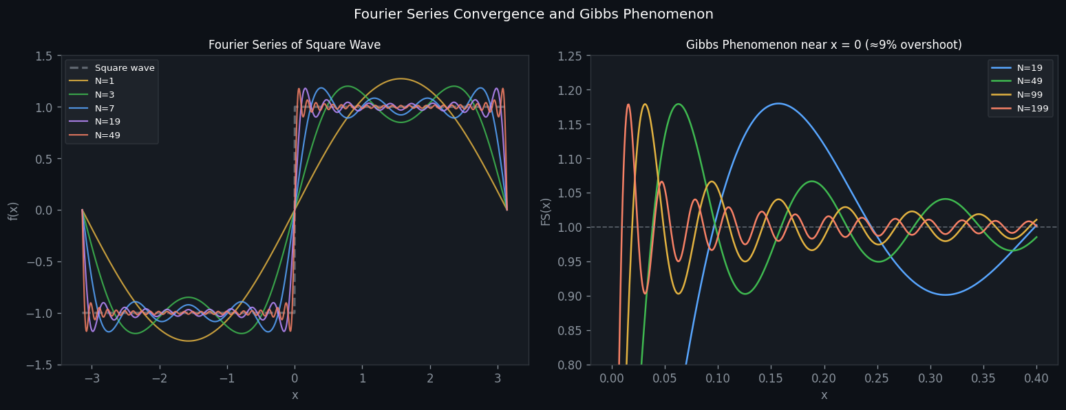
At a jump discontinuity, the partial sums of the Fourier series do not converge uniformly — they exhibit persistent oscillations near the jump known as the Gibbs phenomenon (also called “ringing”).
Specifically, no matter how many terms are included, the partial sums overshoot and undershoot the true function by approximately \(9\%\) of the jump magnitude. These oscillations are not a failure of convergence; the series does converge pointwise (as stated above), but the convergence is not uniform near the jump.
In image processing. A digital image edge is a jump discontinuity in the image function \(f(x,y)\). When a 2D Fourier series is truncated (keeping only low-frequency terms), the ringing appears as “halos” or “ghost lines” around edges. In the Boat test image, truncating Fourier coefficients at varying frequencies \(n = 160, 200, 220, 240\) shows progressively worse ringing around masts and rigging. This is why JPEG-compressed images sometimes display visible artifacts near sharp edges.
Even and Odd Functions
A key simplification arises when \(f\) has symmetry:
- If \(f\) is even (\(f(-x) = f(x)\)): all \(b_n = 0\), and \(a_n = (2/\pi)\int_0^\pi f(x)\cos(nx)\, dx\). The series is a cosine series.
- If \(f\) is odd (\(f(-x) = -f(x)\)): all \(a_n = 0\), and \(b_n = (2/\pi)\int_0^\pi f(x)\sin(nx)\, dx\). The series is a sine series.
Any function can be uniquely decomposed into its even and odd parts: \(f = f_e + f_o\), where \(f_e(x) = [f(x) + f(-x)]/2\) and \(f_o(x) = [f(x) - f(-x)]/2\).
Even/odd extensions. Given a function \(f\) on \([0,\pi]\), its even extension \(f_e\) to \([-\pi, \pi]\) has a cosine series; its odd extension \(f_o\) has a sine series. These are used to solve PDEs on \([0, L]\) with specific boundary conditions.
Illustration. For \(f(x) = x\) on \([0, \pi]\):
- Odd extension to \([-\pi, \pi]\): \(f(x) = 2\sum_{n=1}^\infty (-1)^{n+1} \sin(nx)/n\). Many terms are needed for a good approximation since the function (periodically extended) has jump discontinuities at \(\pm\pi\).
- Even extension: \(f(x) = \pi/2 - (4/\pi)\sum_{k=0}^\infty \cos((2k+1)x)/(2k+1)^2\). Faster convergence since the extended function is continuous.
Parseval’s Identity
This is the function-space analogue of the Pythagorean theorem: the “energy” (squared \(L^2\) norm) of \(f\) equals the sum of squares of its Fourier coefficients. It implies that:
- The Fourier coefficients of a square-integrable function tend to zero: \(a_n, b_n \to 0\) as \(n \to \infty\) (the Riemann-Lebesgue Lemma).
- The Fourier series converges in the \(L^2\) sense (mean-square convergence), even for functions with discontinuities.
Chapter 11: Complex Fourier Series and the Frequency Spectrum
The Complex Exponential Form
Using Euler’s formula \(e^{in x} = \cos(nx) + i\sin(nx)\), we can write
\[ \cos(nx) = \frac{e^{inx} + e^{-inx}}{2}, \quad \sin(nx) = \frac{e^{inx} - e^{-inx}}{2i}. \]Substituting into the real Fourier series and collecting terms in \(e^{inx}\):
The orthogonality relation is:
\[ \frac{1}{2\pi}\int_{-\pi}^{\pi} e^{imx} e^{-inx}\, dx = \delta_{mn}, \]where \(\delta_{mn}\) is the Kronecker delta.
Relationship Between Real and Complex Coefficients
For a real-valued function \(f\):
\[ c_0 = \frac{a_0}{2}, \quad c_n = \frac{a_n - ib_n}{2}, \quad c_{-n} = \frac{a_n + ib_n}{2} = \overline{c_n} \quad (n \geq 1). \]The magnitude: \(|c_n| = |c_{-n}| = \frac{1}{2}\sqrt{a_n^2 + b_n^2}\).
The Frequency Spectrum
The amplitude spectrum is the plot of \(|c_n|\) versus integer \(n\) (or equivalently, versus frequency \(f = n/(2\pi)\)). It displays how much of each frequency is present in the signal.
For a real signal, the spectrum is symmetric about \(n = 0\) since \(|c_n| = |c_{-n}|\). The spectrum is discrete (a set of “spikes” at integer frequencies) for periodic signals.
Fourier Analysis of Music
The connection to music is one of the most beautiful applications of Fourier analysis. A musical note played on an instrument produces a periodic sound wave that is a superposition of many frequencies:
- The fundamental frequency \(f_1 = 1/T\) (where \(T\) is the period) determines the pitch of the note.
- The harmonics at frequencies \(f_k = k \cdot f_1\) (\(k = 2, 3, 4, \ldots\)) give the note its timbre (tone colour).
For example, the note A below middle C has fundamental frequency \(f_1 = 440\) Hz, second harmonic at 880 Hz, third at 1320 Hz, and so on. Two instruments playing the same note have the same fundamental frequency but different distributions of energy among the harmonics — different amplitude spectra — which is why a flute and a clarinet sound different even at the same pitch.
The Fourier coefficients \(|c_n|\) of a single period of the sound wave give precisely the amplitude of the \(n\)-th harmonic. A flute produces mostly the fundamental with small harmonics; an oboe has much richer harmonic content. The human ear acts as a Fourier analyser, decomposing sound into frequency components.
The mathematical framework is: a periodic waveform \(x(t)\) (air pressure variation at the ear) can be written as
\[ x(t) = \sum_{k=0}^\infty A_k \cos(2\pi f_k t) + B_k \sin(2\pi f_k t), \]where \(f_k = k/T\). The Fourier coefficients \(A_k, B_k\) (or equivalently the amplitudes \(|c_k|\)) determine the timbre.
2D Fourier Series and Image Processing
A greyscale image \(f(x,y)\) defined on a square can be expanded as a 2D Fourier series:
\[ f(x,y) = \sum_{m,n=-\infty}^{\infty} c_{mn}\, e^{imx} e^{iny}, \]with coefficients \(c_{mn} = (1/4\pi^2)\iint f(x,y) e^{-imx}e^{-iny}\, dx\, dy\).
The spatial frequency \((m, n)\) corresponds to a pattern that oscillates \(m\) times per unit length in \(x\) and \(n\) times in \(y\). Low-frequency components (\(|m|, |n|\) small) capture the overall brightness and broad structure; high-frequency components capture fine detail and edges.
Gibbs in 2D. At an image edge — a jump discontinuity in \(f(x,y)\) — the 2D Fourier series exhibits 2D Gibbs ringing. When high-frequency Fourier components are removed (as in JPEG compression with aggressive quantisation), the ringing manifests as visible “halos” or “ghost lines” around edges. This is directly observed in the Boat image: truncating at \(n = 160\) vs. \(n = 240\) shows dramatically increasing ringing around sharp edges like the boat masts.
Parseval’s Theorem in Complex Form
In the complex form, Parseval’s identity becomes:
\[ \frac{1}{2\pi}\int_{-\pi}^{\pi} |f(x)|^2\, dx = \sum_{n=-\infty}^{\infty} |c_n|^2. \]The total energy of the signal equals the sum of squared amplitudes over all frequencies. This is the fundamental energy decomposition of the signal. It says: the energy is partitioned among the frequency components, and each frequency contributes independently.
Chapter 12: Applications of Fourier Series
Parseval’s Theorem and Energy Distribution
Parseval’s theorem (Chapter 10–11) tells us how energy is distributed across frequencies. In the complex form:
\[ \frac{1}{2\pi}\int_{-\pi}^{\pi} |f(x)|^2\, dx = \sum_{n=-\infty}^{\infty} |c_n|^2. \]The term \(|c_n|^2\) is the power contributed by the frequency \(n\). For a real signal, the spectrum of \(|c_n|^2\) vs. \(n\) is the power spectrum or periodogram.
Application. For a square wave (alternating between \(\pm 1\)):
\[ f(x) = \frac{4}{\pi}\sum_{k=0}^\infty \frac{\sin((2k+1)x)}{2k+1}. \]The amplitudes \(b_{2k+1} = 4/((2k+1)\pi)\) fall off as \(1/n\), so the energy \(\sum b_n^2\) converges (confirming \(f \in L^2\)), but slowly — the high harmonics carry a noticeable share of the energy. This slow decay is related to the discontinuities of the square wave.
The Heat Equation: Solution via Fourier Series
The derivation of the heat equation in Chapter 8 showed:
\[ \frac{\partial T}{\partial t} = \kappa\, \frac{\partial^2 T}{\partial x^2}, \quad x \in [-\pi, \pi], \quad T(x,0) = f(x). \]This is the one-dimensional heat equation for a thin rod of length \(2\pi\), with initial temperature distribution \(f(x)\).
Fourier’s original insight was to solve this by expanding \(T(x,t)\) as a Fourier series with time-dependent coefficients:
\[ T(x,t) = \frac{a_0(t)}{2} + \sum_{n=1}^\infty \bigl[a_n(t)\cos(nx) + b_n(t)\sin(nx)\bigr]. \]At \(t = 0\): \(a_n(0) = A_n\), \(b_n(0) = B_n\), the Fourier coefficients of \(f\).
Substitution into the Heat Equation
Differentiating the expansion termwise (assuming this is permissible — a technical point addressed in AMATH 353):
\[ \frac{\partial T}{\partial t} = \frac{a_0'(t)}{2} + \sum_{n=1}^\infty \bigl[a_n'(t)\cos(nx) + b_n'(t)\sin(nx)\bigr], \]\[ \frac{\partial^2 T}{\partial x^2} = -\sum_{n=1}^\infty n^2 \bigl[a_n(t)\cos(nx) + b_n(t)\sin(nx)\bigr]. \]Substituting into the heat equation and collecting like terms (by linear independence of \(\{\cos(nx), \sin(nx)\}\)):
\[ a_0'(t) = 0 \implies a_0(t) = A_0 = \text{const}, \]\[ a_n'(t) + \kappa n^2 a_n(t) = 0, \quad b_n'(t) + \kappa n^2 b_n(t) = 0, \quad n \geq 1. \]These are first-order linear ODEs with solutions:
\[ a_n(t) = A_n\, e^{-\kappa n^2 t}, \quad b_n(t) = B_n\, e^{-\kappa n^2 t}. \]The Solution
\[ \boxed{T(x,t) = \frac{A_0}{2} + \sum_{n=1}^\infty e^{-\kappa n^2 t}\bigl[A_n\cos(nx) + B_n\sin(nx)\bigr],} \]where \(A_n, B_n\) are the Fourier coefficients of the initial temperature \(f(x)\).
Equivalently, in complex form:
\[ T(x,t) = \sum_{n=-\infty}^{\infty} c_n\, e^{inx}\, e^{-\kappa n^2 t}, \]where \(c_n\) are the complex Fourier coefficients of \(f\).
Physical Interpretation
The solution reveals the remarkable physics of heat diffusion:
Exponential decay of harmonics. Every frequency component \(n\) decays by the factor \(e^{-\kappa n^2 t}\). The decay rate \(\kappa n^2\) grows quadratically with frequency. High-frequency components decay much faster than low-frequency components.
Smoothing in time. At any \(t > 0\), all the Fourier coefficients have been multiplied by \(e^{-\kappa n^2 t} < 1\), so the series converges much better than the series for \(f\) itself. Even if \(f\) has jump discontinuities (requiring slowly decaying Fourier coefficients), \(T(x,t)\) is instantaneously smooth for any \(t > 0\). Heat diffusion is a smoothing process.
Long-time behaviour. As \(t \to \infty\), all terms with \(n \geq 1\) decay to zero:
The rod reaches a uniform temperature equal to the average of the initial temperature distribution. Heat has been redistributed from hotter to cooler regions until equilibrium. The total heat energy is conserved (it has just been redistributed).
- Physical connection. The factor \(\kappa = k/(c\rho)\) determines the timescale. A good thermal conductor (large \(k\)) equilibrates quickly; a poor conductor (small \(k\)) retains temperature gradients much longer.
Legendre Polynomials and Other Orthogonal Systems
Fourier series are a particular example of the general theory of orthogonal function expansions. In this framework, one replaces the trigonometric functions with other orthogonal families suited to the geometry of the problem.
The Legendre polynomials \(\{P_n(x)\}_{n=0}^\infty\) are orthogonal on \([-1, 1]\):
\[ \int_{-1}^{1} P_m(x) P_n(x)\, dx = \frac{2}{2n+1}\, \delta_{mn}. \]They arise naturally in solving Laplace’s equation \(\nabla^2 f = 0\) in spherical coordinates via separation of variables. The solutions are the spherical harmonics \(Y_n^m(\theta, \phi)\), built from Legendre polynomials, which describe the angular dependence of quantum mechanical wavefunctions for the hydrogen atom (AMATH 373) and solutions to Laplace’s equation in 3D.
Similarly, Bessel functions arise for problems with cylindrical symmetry, Chebyshev polynomials are optimal for polynomial approximation, and Hermite polynomials appear in quantum mechanics (harmonic oscillator). All share the key property of orthogonality with respect to a suitable inner product (possibly with a weight function), enabling coefficient extraction by inner products — the same technique as for Fourier series.
The abstract framework that unifies all these examples is the theory of Hilbert spaces, which you will encounter in AMATH 351/353, PMATH 450, and AMATH 373. The function space \(L^2\) from this course is the prototype.
The Wave Equation and Plucked String
A brief preview: the Fourier method applies equally to the wave equation:
\[ u_{tt} = c^2 u_{xx}, \quad x \in (0, L), \quad u(0,t) = u(L,t) = 0. \]This models a vibrating string (guitar string, violin string) with fixed endpoints. Assuming a separation-of-variables solution \(u(x,t) = X(x)T(t)\), one finds that the spatial functions satisfying the boundary conditions are \(X_n(x) = \sin(n\pi x/L)\), and the time dependence is \(T_n(t) = a_n\cos(n\pi ct/L) + b_n\sin(n\pi ct/L)\).
The general solution is a Fourier sine series:
\[ u(x,t) = \sum_{n=1}^\infty \sin\!\left(\frac{n\pi x}{L}\right)\!\left[a_n\cos\!\left(\frac{n\pi c}{L}t\right) + b_n\sin\!\left(\frac{n\pi c}{L}t\right)\right], \]where \(a_n, b_n\) are determined by the initial displacement and velocity.
The frequencies \(f_n = nc/(2L)\) are the normal modes or harmonics: the fundamental at \(f_1 = c/(2L)\) and overtones at \(f_2, f_3, \ldots\). This is precisely the mathematical explanation of why musical instruments produce harmonics: the physical constraint of fixed endpoints forces the vibrations to be Fourier modes.
Summary: The Architecture of the Course
This course built upward through two interlocking structures.
Vector calculus moved from the differential operators (gradient, divergence, curl) to the integral theorems. The gradient connects scalar fields to their geometry. Divergence and curl extract the “spreading” and “spinning” of vector fields. The Fundamental Theorem for Line Integrals, Green’s Theorem, the Divergence Theorem, and Stokes’ Theorem are four versions of the same principle: an integral over a domain equals an integral over its boundary, with the right differential operator applied. These theorems unify much of physics — Maxwell’s equations, the continuity equation, the heat equation, and the conservation laws of mechanics all fall naturally from this framework.
Fourier analysis translated the problem of function decomposition into the language of infinite-dimensional linear algebra. The orthogonality of sines and cosines — a consequence of simple integral identities — enables the extraction of frequency components. Parseval’s theorem guarantees that the decomposition conserves energy. The heat equation solution brought both halves of the course together: Fourier series, derived from the trigonometric orthogonal basis, provide the eigenfunctions of the Laplacian that appear in the heat equation derived via the Divergence Theorem.
Together, these tools form the mathematical foundation for AMATH 353 (PDEs), AMATH 361 (continuum mechanics), AMATH 391 (wavelets), PHYS 252/253 (electromagnetism), and AMATH 373 (quantum mechanics).
