STAT 230: Probability
Estimated study time: 45 minutes
Table of contents
Chapter 1: Introduction to Probability
Probability theory provides mathematical tools for quantifying uncertainty and variability. There are three classical ways to think about the probability of an event: the classical definition (ratio of favourable to total equally likely outcomes), the relative frequency definition (long-run proportion in repeated trials), and the subjective probability definition (a personal measure of belief). Each has limitations, so the modern approach treats probability axiomatically.
The mathematical framework we develop rests on three components: a sample space of all possible outcomes, a collection of events (subsets of the sample space) to which probabilities are assigned, and a rule for assigning probabilities consistent with certain axioms.
Chapter 2: Mathematical Probability Models
2.1 Sample Spaces and Probability
Definition 1 (Sample Space). A sample space \(S\) is a set of distinct outcomes for an experiment or process, with the property that in a single trial, one and only one of these outcomes occurs.
A sample space is discrete if it consists of a finite or countably infinite set of outcomes. A sample space is not necessarily unique for a given experiment; the choice depends on what aspects of the experiment matter for the problem at hand.
Definition 2 (Event). An event in a discrete sample space is a subset \(A \subseteq S\). If the event contains only one point, e.g. \(A_1 = \{a_1\}\), it is called a simple event. An event made up of two or more simple events is called a compound event.
Definition 3 (Probability Distribution on a Discrete Sample Space). Let \(S = \{a_1, a_2, a_3, \ldots\}\) be a discrete sample space. Assign probabilities \(P(a_i)\) to the outcomes such that:
- \(0 \le P(a_i) \le 1\) for all \(i\),
- \(\sum_{\text{all } i} P(a_i) = 1\).
The collection \(\{P(a_i)\}\) is called a probability distribution on \(S\).
Definition 4 (Probability of an Event). The probability \(P(A)\) of an event \(A\) is the sum of the probabilities of all the simple events that make up \(A\):
\[ P(A) = \sum_{a \in A} P(a). \]For discrete sample spaces with equally likely outcomes (\(P(a_i) = 1/n\) for all \(i\)), computing \(P(A)\) reduces to counting: \(P(A) = |A|/|S|\).
Definition 5 (Odds). The odds in favour of an event \(A\) is \(\frac{P(A)}{1 - P(A)}\). The odds against the event is the reciprocal, \(\frac{1 - P(A)}{P(A)}\).
Chapter 3: Probability and Counting Techniques
When the sample space has equally likely outcomes, probability calculations reduce to counting. This chapter develops the key counting tools.
3.1 Addition and Multiplication Rules
- Addition Rule: If job 1 can be done in \(p\) ways and job 2 in \(q\) ways, then we can do job 1 OR job 2 (but not both) in \(p + q\) ways.
- Multiplication Rule: If job 1 can be done in \(p\) ways and, for each of these, job 2 in \(q\) ways, then both job 1 AND job 2 can be done in \(p \times q\) ways.
The association “OR \(\leftrightarrow\) addition” and “AND \(\leftrightarrow\) multiplication” recurs throughout probability.
3.2 Counting Arrangements or Permutations
Starting with \(n\) distinct symbols:
- The number of arrangements of all \(n\) symbols is \(n!\).
- The number of arrangements of length \(k\) (each symbol used at most once) is \(n^{(k)} = \frac{n!}{(n-k)!}\).
- The number of arrangements of length \(k\) with replacement is \(n^k\).
Stirling’s Approximation: For large \(n\), \(n! \approx (n/e)^n \sqrt{2\pi n}\).
3.3 Counting Subsets or Combinations
The number of subsets of size \(k\) chosen from \(n\) objects is
\[ \binom{n}{k} = \frac{n!}{k!(n-k)!} = \frac{n^{(k)}}{k!}. \]Key properties include \(\binom{n}{k} = \binom{n}{n-k}\) and \(\binom{n}{k} = \binom{n-1}{k-1} + \binom{n-1}{k}\) (Pascal’s identity).
Binomial Theorem: \((1+x)^n = \sum_{k=0}^{n} \binom{n}{k} x^k\).
3.4 Arrangements with Repeated Symbols
If we have \(n\) symbols total with \(n_i\) of type \(i\) (for \(i = 1, 2, \ldots, k\)) where \(n_1 + n_2 + \cdots + n_k = n\), the number of distinct arrangements is
\[ \frac{n!}{n_1! \, n_2! \cdots n_k!}. \]Chapter 4: Probability Rules and Conditional Probability
4.1 General Methods
The basic rules of probability follow directly from the definitions:
- Rule 1: \(P(S) = 1\).
- Rule 2: For any event \(A\), \(0 \le P(A) \le 1\).
- Rule 3: If \(A \subseteq B\) then \(P(A) \le P(B)\).
De Morgan’s Laws relate complements and set operations:
\[ \overline{A \cup B} = \bar{A} \cap \bar{B}, \qquad \overline{A \cap B} = \bar{A} \cup \bar{B}. \]4.2 Rules for Unions of Events
Rule 4a (Addition Law / Inclusion-Exclusion for Two Events).
\[ P(A \cup B) = P(A) + P(B) - P(A \cap B). \]Rule 4b (Inclusion-Exclusion for Three Events).
\[ P(A \cup B \cup C) = P(A) + P(B) + P(C) - P(AB) - P(AC) - P(BC) + P(ABC). \]Rule 4c (Inclusion-Exclusion for \(n\) Events).
\[ P\!\left(\bigcup_{i=1}^n A_i\right) = \sum_i P(A_i) - \sum_{iDefinition 6 (Mutually Exclusive Events). Events \(A\) and \(B\) are mutually exclusive if \(A \cap B = \emptyset\). More generally, \(A_1, \ldots, A_n\) are mutually exclusive if \(A_i \cap A_j = \emptyset\) for all \(i \ne j\).
Rule 5a. If \(A\) and \(B\) are mutually exclusive, \(P(A \cup B) = P(A) + P(B)\).
Rule 5b. If \(A_1, \ldots, A_n\) are mutually exclusive, \(P(A_1 \cup \cdots \cup A_n) = \sum_{i=1}^n P(A_i)\).
Rule 6 (Complement Rule). \(P(\bar{A}) = 1 - P(A)\).
4.3 Intersections of Events and Independence
Definition 7 (Independent Events). Events \(A\) and \(B\) are independent if and only if \(P(A \cap B) = P(A)P(B)\). If not independent, they are called dependent.
Definition 8 (Mutual Independence). Events \(A_1, A_2, \ldots, A_n\) are mutually independent if and only if
\[ P(A_{i_1} \cap A_{i_2} \cap \cdots \cap A_{i_k}) = P(A_{i_1})P(A_{i_2}) \cdots P(A_{i_k}) \]for every subset \(\{i_1, i_2, \ldots, i_k\}\) of distinct indices from \(\{1, 2, \ldots, n\}\).
Mutual independence requires checking all \(2^n - n - 1\) subset conditions, not just pairwise independence. If \(A\) and \(B\) are independent, then \(\bar{A}\) and \(B\) are also independent (and similarly for other complement combinations).
4.4 Conditional Probability
Definition 9 (Conditional Probability). The conditional probability of event \(A\), given event \(B\), is
\[ P(A \mid B) = \frac{P(A \cap B)}{P(B)}, \quad \text{provided } P(B) > 0. \]If \(A\) and \(B\) are independent, then \(P(A \mid B) = P(A)\).
Theorem 10. Suppose \(A\) and \(B\) are events with \(P(A) > 0\) and \(P(B) > 0\). Then \(A\) and \(B\) are independent if and only if either \(P(A \mid B) = P(A)\) or \(P(B \mid A) = P(B)\).
4.5 Product Rules, Law of Total Probability, and Bayes’ Theorem
Rule 7 (Product Rules). For events \(A, B, C, D, \ldots\) with appropriate positive probabilities:
\[ P(AB) = P(A)P(B \mid A), \]\[ P(ABC) = P(A)P(B \mid A)P(C \mid AB), \]\[ P(ABCD) = P(A)P(B \mid A)P(C \mid AB)P(D \mid ABC), \]and so on.
Rule 8 (Law of Total Probability). Let \(A_1, A_2, \ldots, A_k\) be a partition of \(S\) (i.e., mutually exclusive events whose union is \(S\)). For any event \(B\),
\[ P(B) = \sum_{i=1}^k P(B \mid A_i) P(A_i). \]Bayes’ Theorem. Suppose \(P(B) > 0\). Then
\[ P(A \mid B) = \frac{P(B \mid A)P(A)}{P(B)} = \frac{P(B \mid A)P(A)}{P(B \mid A)P(A) + P(B \mid \bar{A})P(\bar{A})}. \]More generally, if \(A_1, \ldots, A_k\) partition \(S\),
\[ P(A_i \mid B) = \frac{P(B \mid A_i)P(A_i)}{\sum_{j=1}^k P(B \mid A_j)P(A_j)}. \]4.6 Useful Series and Sums
The following identities are used frequently in later chapters:
- Geometric Series: \(\sum_{x=0}^{\infty} t^x = \frac{1}{1-t}\) for \(|t| < 1\).
- Binomial Theorem (integer \(n\)): \((1+t)^n = \sum_{x=0}^n \binom{n}{x} t^x\).
- Generalized Binomial Theorem (real \(n\)): \((1+t)^n = \sum_{x=0}^{\infty} \binom{n}{x} t^x\) for \(|t| < 1\).
- Multinomial Theorem: \((t_1 + \cdots + t_k)^n = \sum \frac{n!}{x_1! \cdots x_k!} t_1^{x_1} \cdots t_k^{x_k}\).
- Hypergeometric Identity: \(\sum_x \binom{a}{x}\binom{b}{n-x} = \binom{a+b}{n}\).
- Exponential Series: \(e^t = \sum_{n=0}^{\infty} \frac{t^n}{n!}\).
Chapter 5: Discrete Random Variables
5.1 Random Variables and Probability Functions
Definition 11 (Random Variable). A random variable is a function that assigns a real number to each point in a sample space \(S\).
Random variables are classified as discrete (taking values in a countable set) or continuous (taking values in an interval of real numbers).
Definition 12 (Probability Function). Let \(X\) be a discrete random variable with \(\text{range}(X) = A\). The probability function (p.f.) of \(X\) is
\[ f(x) = P(X = x), \quad \text{defined for all } x \in A. \]The set of pairs \(\{(x, f(x)) : x \in A\}\) is called the probability distribution of \(X\). Every probability function satisfies: (1) \(f(x) \ge 0\) for all \(x \in A\), and (2) \(\sum_{x \in A} f(x) = 1\).
Definition 13 (Cumulative Distribution Function). The cumulative distribution function (c.d.f.) of \(X\) is
\[ F(x) = P(X \le x) = \sum_{u \le x} f(u), \quad \text{defined for all } x \in \mathbb{R}. \]Properties: (1) \(F(x)\) is non-decreasing, (2) \(0 \le F(x) \le 1\), (3) \(\lim_{x \to -\infty} F(x) = 0\) and \(\lim_{x \to \infty} F(x) = 1\).
For integer-valued random variables, \(f(x) = F(x) - F(x-1)\).
5.2 Discrete Uniform Distribution
Physical Setup: \(X\) takes values \(a, a+1, \ldots, b\) with all values equally likely.
Discrete Uniform Distribution. If \(X \sim \text{Uniform}\{a, a+1, \ldots, b\}\), then
\[ f(x) = \frac{1}{b - a + 1}, \quad x = a, a+1, \ldots, b. \]5.3 Hypergeometric Distribution
Physical Setup: A collection of \(N\) objects contains \(r\) successes and \(N - r\) failures. We select \(n\) objects at random without replacement. Let \(X\) = number of successes obtained.
Hypergeometric Distribution.
\[ f(x) = P(X = x) = \frac{\binom{r}{x}\binom{N-r}{n-x}}{\binom{N}{n}}, \quad x = \max(0, n - N + r), \ldots, \min(n, r). \]5.4 Binomial Distribution
Physical Setup: An experiment with two outcomes (S with probability \(p\), F with probability \(1-p\)) is repeated \(n\) independent times. Let \(X\) = number of successes. Then \(X \sim \text{Binomial}(n, p)\).
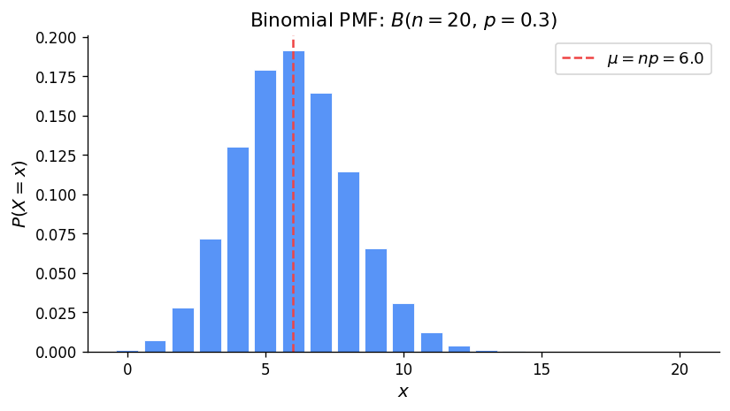
Binomial Distribution.
\[ f(x) = P(X = x) = \binom{n}{x} p^x (1-p)^{n-x}, \quad x = 0, 1, 2, \ldots, n. \]Binomial vs. Hypergeometric: The Binomial requires independent trials (constant \(p\)), while the Hypergeometric involves sampling without replacement. When \(N\) is large relative to \(n\), the Binomial approximates the Hypergeometric well.
5.5 Negative Binomial Distribution
Physical Setup: Repeat independent Bernoulli trials (each with probability \(p\) of success) until the \(k\)-th success. Let \(X\) = number of failures before the \(k\)-th success. Then \(X \sim NB(k, p)\).
Negative Binomial Distribution.
\[ f(x) = P(X = x) = \binom{x+k-1}{x} p^k (1-p)^x, \quad x = 0, 1, 2, \ldots \]Binomial vs. Negative Binomial: In the Binomial, \(n\) (number of trials) is fixed and \(X\) (successes) is random. In the Negative Binomial, \(k\) (successes) is fixed and the number of trials is random.
5.6 Geometric Distribution
Physical Setup: The special case of the Negative Binomial with \(k = 1\). Repeat independent Bernoulli trials until the first success; let \(X\) = number of failures before the first success. Then \(X \sim \text{Geometric}(p)\).
Geometric Distribution.
\[ f(x) = P(X = x) = p(1-p)^x, \quad x = 0, 1, 2, \ldots \]The Geometric distribution has the memoryless property: \(P(X \ge s + t \mid X \ge s) = P(X \ge t)\).
5.7 Poisson Distribution from Binomial
The Poisson distribution arises as a limit of \(\text{Binomial}(n, p)\) when \(n \to \infty\), \(p \to 0\), and \(np = \mu\) is held fixed.
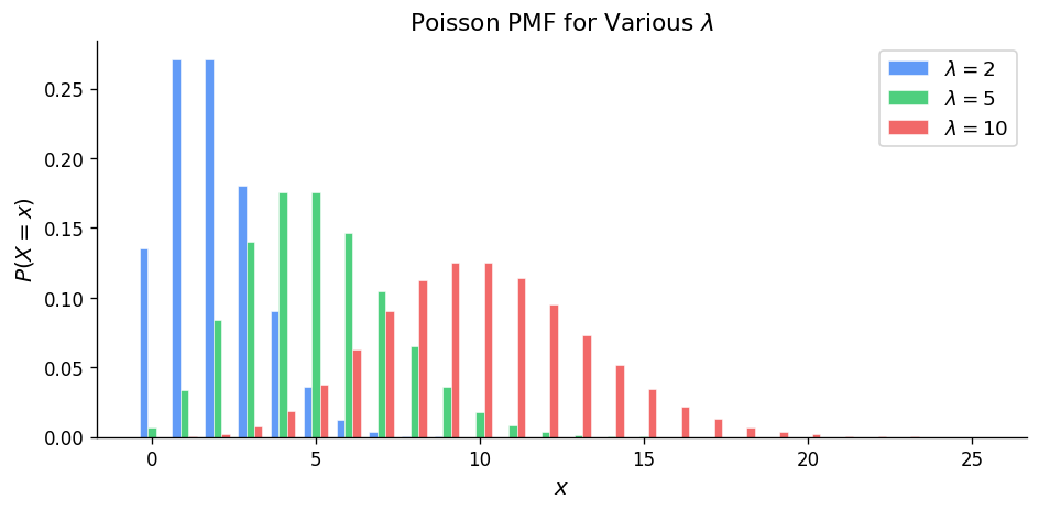
Poisson Distribution. If \(X \sim \text{Poisson}(\mu)\), then
\[ f(x) = P(X = x) = \frac{e^{-\mu} \mu^x}{x!}, \quad x = 0, 1, 2, \ldots \]where \(\mu > 0\).
The Poisson distribution provides a good approximation to \(\text{Binomial}(n, p)\) when \(n\) is large and \(p\) is small, with \(\mu = np\).
5.8 Poisson Distribution from Poisson Process
A Poisson process is defined by three conditions:
- Independence: Numbers of occurrences in non-overlapping intervals are independent.
- Individuality: \(P(\text{2 or more events in } (t, t + \Delta t)) = o(\Delta t)\) as \(\Delta t \to 0\).
- Homogeneity: \(P(\text{one event in } (t, t + \Delta t)) = \lambda \Delta t + o(\Delta t)\).
If events follow a Poisson process with rate \(\lambda\), the number of events \(X\) in a time interval of length \(t\) has distribution \(X \sim \text{Poisson}(\mu)\) with \(\mu = \lambda t\). Here \(\lambda\) is the average rate of occurrence per unit time.
The Poisson process also applies to events in space (area or volume), with \(\mu = \lambda v\) where \(v\) is the size of the region.
5.10 Summary of Discrete Distributions
| Distribution | \(f(x)\) | Range | Mean | Variance |
|---|---|---|---|---|
| Discrete Uniform | \(\frac{1}{b-a+1}\) | \(x = a, \ldots, b\) | \(\frac{a+b}{2}\) | \(\frac{(b-a+1)^2 - 1}{12}\) |
| Hypergeometric | \(\frac{\binom{r}{x}\binom{N-r}{n-x}}{\binom{N}{n}}\) | \(\max(0,n\!-\!N\!+\!r) \le x \le \min(n,r)\) | \(\frac{nr}{N}\) | \(\frac{nr(N-r)(N-n)}{N^2(N-1)}\) |
| Binomial\((n,p)\) | \(\binom{n}{x}p^x(1-p)^{n-x}\) | \(x = 0, 1, \ldots, n\) | \(np\) | \(np(1-p)\) |
| Negative Binomial\((k,p)\) | \(\binom{x+k-1}{x}p^k(1-p)^x\) | \(x = 0, 1, 2, \ldots\) | \(\frac{k(1-p)}{p}\) | \(\frac{k(1-p)}{p^2}\) |
| Geometric\((p)\) | \(p(1-p)^x\) | \(x = 0, 1, 2, \ldots\) | \(\frac{1-p}{p}\) | \(\frac{1-p}{p^2}\) |
| Poisson\((\mu)\) | \(\frac{e^{-\mu}\mu^x}{x!}\) | \(x = 0, 1, 2, \ldots\) | \(\mu\) | \(\mu\) |
Chapter 7: Expected Value and Variance
7.1 Summarizing Data on Random Variables
Definition 14 (Median). The median of a sample is a value such that half the results are below it and half above it, when the results are arranged in numerical order.
Definition 15 (Mode). The mode of a sample is the value which occurs most often. There may be more than one mode.
7.2 Expectation of a Random Variable
Definition 16 (Expected Value). Let \(X\) be a discrete random variable with \(\text{range}(X) = A\) and probability function \(f(x)\). The expected value (mean, expectation) of \(X\) is
\[ E(X) = \mu = \sum_{x \in A} x \, f(x). \]Theorem 17 (Expected Value of a Function). Let \(X\) be a discrete random variable. The expected value of a function \(g(X)\) is
\[ E[g(X)] = \sum_{x \in A} g(x) f(x). \]Linearity of Expectation: For constants \(a\) and \(b\),
\[ E[ag(X) + b] = aE[g(X)] + b. \]More generally, \(E[ag_1(X) + bg_2(X)] = aE[g_1(X)] + bE[g_2(X)]\).
Note that in general \(E[g(X)] \ne g(E[X])\) for nonlinear \(g\).
7.4 Means and Variances of Distributions
Definition 18 (Variance). The variance of a random variable \(X\) is
\[ \sigma^2 = \text{Var}(X) = E[(X - \mu)^2]. \]Two useful computational formulas:
- \(\text{Var}(X) = E(X^2) - [E(X)]^2\)
- \(\text{Var}(X) = E[X(X-1)] + E(X) - [E(X)]^2\)
Definition 19 (Standard Deviation).
\[ \sigma = \text{sd}(X) = \sqrt{\text{Var}(X)}. \]Properties of Mean and Variance under linear transformation: If \(Y = aX + b\), then
\[ E(Y) = aE(X) + b, \qquad \text{Var}(Y) = a^2 \text{Var}(X). \]Derivations of Mean and Variance for Key Distributions
Binomial: \(E(X) = np\), \(\text{Var}(X) = np(1-p)\).
Poisson: \(E(X) = \mu\), \(\text{Var}(X) = \mu\) (mean equals variance).
Geometric: \(E(X) = \frac{1-p}{p}\), \(\text{Var}(X) = \frac{1-p}{p^2}\).
Negative Binomial: \(E(X) = \frac{k(1-p)}{p}\), \(\text{Var}(X) = \frac{k(1-p)}{p^2}\).
Hypergeometric: \(E(X) = \frac{nr}{N}\), \(\text{Var}(X) = \frac{nr(N-r)(N-n)}{N^2(N-1)}\).
Chapter 8: Continuous Random Variables
8.1 General Terminology and Notation
For continuous random variables, \(P(X = x) = 0\) for every individual value \(x\); probabilities are assigned to intervals.
The cumulative distribution function \(F(x) = P(X \le x)\) has the same properties as in the discrete case: non-decreasing, \(\lim_{x \to -\infty} F(x) = 0\), \(\lim_{x \to \infty} F(x) = 1\). Since \(P(X = a) = 0\),
\[ P(a < X < b) = P(a \le X \le b) = F(b) - F(a). \]Definition 20 (Probability Density Function). The probability density function (p.d.f.) \(f(x)\) for a continuous random variable \(X\) is
\[ f(x) = \frac{dF(x)}{dx} \]where \(F(x)\) is the cumulative distribution function.
Properties of a p.d.f.: (1) \(f(x) \ge 0\), (2) \(\int_{-\infty}^{\infty} f(x)\,dx = 1\), (3) \(P(a \le X \le b) = \int_a^b f(x)\,dx\), (4) \(F(x) = \int_{-\infty}^x f(u)\,du\).
Note that \(f(x) \ne P(X = x)\), but \(f(x)\,\Delta x \approx P(x - \Delta x/2 \le X \le x + \Delta x/2)\) for small \(\Delta x\).
Definition 21 (Quantiles and Percentiles). The \(p\)th quantile (or \(100p\)th percentile) of a continuous random variable \(X\) is the value \(q(p)\) such that \(P(X \le q(p)) = p\). The median is \(q(0.5)\).
Change of Variable: If \(Y = g(X)\) for a monotone function \(g\), find \(F_Y(y) = P(Y \le y)\) by expressing the event in terms of \(X\), then differentiate to get \(f_Y(y)\).
Definition 22 (Expectation for Continuous Random Variables).
\[ E[g(X)] = \int_{-\infty}^{\infty} g(x) f(x)\,dx. \]In particular, \(\mu = E(X) = \int_{-\infty}^{\infty} x f(x)\,dx\) and \(\text{Var}(X) = E(X^2) - \mu^2\).
All earlier properties of expectation and variance carry over to continuous random variables.
8.2 Continuous Uniform Distribution
Physical Setup: \(X\) takes values in \([a, b]\) with all subintervals of a fixed length being equally likely. Write \(X \sim U(a, b)\).
Continuous Uniform Distribution.
\[ f(x) = \frac{1}{b-a}, \quad a \le x \le b; \qquad F(x) = \frac{x - a}{b - a}, \quad a \le x \le b. \]\[ E(X) = \frac{a+b}{2}, \qquad \text{Var}(X) = \frac{(b-a)^2}{12}. \]8.3 Exponential Distribution
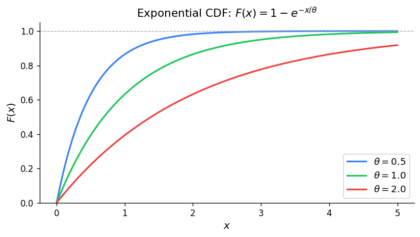
Physical Setup: In a Poisson process with rate \(\lambda\), let \(X\) be the waiting time until the first event. Then \(X \sim \text{Exponential}(\theta)\) where \(\theta = 1/\lambda\).
Exponential Distribution. If \(X \sim \text{Exponential}(\theta)\), then
\[ f(x) = \frac{1}{\theta} e^{-x/\theta}, \quad x > 0; \qquad F(x) = 1 - e^{-x/\theta}, \quad x > 0. \]\[ E(X) = \theta, \qquad \text{Var}(X) = \theta^2. \]Definition 23 (Gamma Function).
\[ \Gamma(\alpha) = \int_0^{\infty} y^{\alpha - 1} e^{-y}\,dy, \quad \alpha > 0. \]Key properties: \(\Gamma(\alpha) = (\alpha - 1)\Gamma(\alpha - 1)\) for \(\alpha > 1\), \(\Gamma(n+1) = n!\) for non-negative integers, \(\Gamma(1/2) = \sqrt{\pi}\).
Memoryless Property: \(P(X > c + b \mid X > b) = P(X > c)\). Given that you have already waited \(b\) time units, the probability of waiting an additional \(c\) units does not depend on \(b\).
8.4 Computer Generation of Random Variables
Theorem 24 (Inverse CDF Method). If \(F\) is an arbitrary cumulative distribution function and \(U \sim U(0,1)\), then the random variable \(X = F^{-1}(U)\) has cumulative distribution function \(F(x)\).
This is the standard method for generating non-uniform random variables from uniform ones.
8.5 Normal Distribution
Physical Setup: \(X\) has a Normal distribution if its p.d.f. is the symmetric “bell curve.”
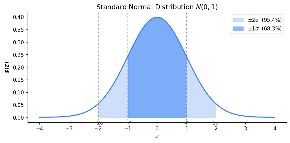
Normal Distribution. If \(X \sim N(\mu, \sigma^2)\), then
\[ f(x) = \frac{1}{\sqrt{2\pi}\,\sigma} \exp\!\left(-\frac{1}{2}\left(\frac{x - \mu}{\sigma}\right)^2\right), \quad x \in \mathbb{R}. \]\[ E(X) = \mu, \qquad \text{Var}(X) = \sigma^2. \]The standard Normal distribution is \(Z \sim N(0, 1)\), with p.d.f. \(\phi(z) = \frac{1}{\sqrt{2\pi}} e^{-z^2/2}\).
Theorem 25 (Standardization). If \(X \sim N(\mu, \sigma^2)\) and \(Z = (X - \mu)/\sigma\), then \(Z \sim N(0, 1)\) and
\[ P(X \le x) = P\!\left(Z \le \frac{x - \mu}{\sigma}\right). \]By symmetry of the standard Normal: \(P(Z \le -z) = P(Z \ge z) = 1 - P(Z \le z)\).
Summary of Continuous Distributions
| Distribution | \(f(x)\) | Mean | Variance |
|---|---|---|---|
| \(U(a,b)\) | \(\frac{1}{b-a}\), \(a \le x \le b\) | \(\frac{a+b}{2}\) | \(\frac{(b-a)^2}{12}\) |
| \(\text{Exponential}(\theta)\) | \(\frac{1}{\theta}e^{-x/\theta}\), \(x > 0\) | \(\theta\) | \(\theta^2\) |
| \(N(\mu, \sigma^2)\) | \(\frac{1}{\sqrt{2\pi}\sigma}e^{-(x-\mu)^2/(2\sigma^2)}\) | \(\mu\) | \(\sigma^2\) |
Chapter 9: Multivariate Distributions
9.1 Basic Terminology and Techniques
For two discrete random variables \(X\) and \(Y\), the joint probability function is \(f(x, y) = P(X = x, Y = y)\). The marginal probability functions are
\[ f_1(x) = \sum_y f(x, y), \qquad f_2(y) = \sum_x f(x, y). \]Definition 26 (Independent Random Variables). \(X\) and \(Y\) are independent random variables if \(f(x, y) = f_1(x) f_2(y)\) for all \((x, y)\).
Definition 27 (Mutual Independence). \(X_1, X_2, \ldots, X_n\) are independent random variables if and only if
\[ f(x_1, x_2, \ldots, x_n) = f_1(x_1) f_2(x_2) \cdots f_n(x_n) \]for all \((x_1, \ldots, x_n)\).
Definition 28 (Conditional Probability Function). The conditional probability function of \(X\) given \(Y = y\) is
\[ f_1(x \mid y) = \frac{f(x, y)}{f_2(y)}, \quad \text{provided } f_2(y) > 0. \]Results for Sums of Independent Random Variables
Theorem 29. If \(X \sim \text{Poisson}(\mu_1)\) and \(Y \sim \text{Poisson}(\mu_2)\) independently, then
\[ T = X + Y \sim \text{Poisson}(\mu_1 + \mu_2). \]Theorem 30. If \(X \sim \text{Binomial}(n, p)\) and \(Y \sim \text{Binomial}(m, p)\) independently, then
\[ T = X + Y \sim \text{Binomial}(n + m, p). \]9.2 Multinomial Distribution
The Multinomial distribution generalizes the Binomial to \(k\) categories. If each of \(n\) independent trials results in outcome \(i\) with probability \(p_i\) (\(i = 1, \ldots, k\), \(\sum p_i = 1\)), and \(X_i\) counts the number of type-\(i\) outcomes, then
\[ P(X_1 = x_1, \ldots, X_k = x_k) = \frac{n!}{x_1! x_2! \cdots x_k!} p_1^{x_1} p_2^{x_2} \cdots p_k^{x_k} \]where \(\sum x_i = n\).
9.3 Markov Chains
A Markov chain is a sequence of random variables \(X_0, X_1, X_2, \ldots\) taking values in a finite state space, such that
\[ P(X_{n+1} = j \mid X_n = i, X_{n-1}, \ldots, X_0) = P(X_{n+1} = j \mid X_n = i) = p_{ij}. \]The matrix \(P = (p_{ij})\) is called the transition matrix. The \(n\)-step transition probabilities are given by \(P^n\).
Definition 31 (Limiting Distribution). A limiting distribution of a Markov chain is a vector \(\pi\) of long-run probabilities such that \(\pi_j = \lim_{n \to \infty} P(X_n = j)\) for all states \(j\), regardless of the initial state.
Definition 32 (Stationary Distribution). A stationary distribution is a probability vector \(\pi\) satisfying \(\pi^T P = \pi^T\).
9.4 Expectation for Multivariate Distributions: Covariance and Correlation
Definition 33 (Expected Value of a Function of Two Variables).
\[ E[g(X, Y)] = \sum_x \sum_y g(x, y) f(x, y). \]Results for Means
\[ E(aX + bY) = aE(X) + bE(Y) \]for any constants \(a, b\). This extends to any linear combination of random variables, whether independent or not.
Definition 34 (Covariance).
\[ \text{Cov}(X, Y) = E[(X - \mu_X)(Y - \mu_Y)] = E(XY) - E(X)E(Y). \]Theorem 35. If \(X\) and \(Y\) are independent, then \(\text{Cov}(X, Y) = 0\).
The converse is not true in general: zero covariance does not imply independence.
Theorem 36. If \(X\) and \(Y\) are independent random variables, then for any functions \(g_1\) and \(g_2\),
\[ E[g_1(X) g_2(Y)] = E[g_1(X)] \cdot E[g_2(Y)]. \]Results for Covariance
- \(\text{Cov}(X, X) = \text{Var}(X)\).
- \(\text{Cov}(X, Y) = \text{Cov}(Y, X)\).
- \(\text{Cov}(aX + b, cY + d) = ac\,\text{Cov}(X, Y)\).
Definition 37 (Correlation Coefficient).
\[ \rho = \text{Corr}(X, Y) = \frac{\text{Cov}(X, Y)}{\sigma_X \sigma_Y} \]where \(-1 \le \rho \le 1\). If \(\rho = 0\), the variables are said to be uncorrelated.
9.5 Mean and Variance of a Linear Combination
Results for Variance
For \(T = a_1 X_1 + a_2 X_2 + \cdots + a_n X_n\):
\[ \text{Var}(T) = \sum_{i=1}^n a_i^2 \text{Var}(X_i) + 2 \sum_{i < j} a_i a_j \text{Cov}(X_i, X_j). \]If \(X_1, \ldots, X_n\) are independent, the covariance terms vanish:
\[ \text{Var}(T) = \sum_{i=1}^n a_i^2 \text{Var}(X_i). \]In particular, for the sample mean \(\bar{X} = \frac{1}{n}\sum X_i\) of i.i.d. random variables with mean \(\mu\) and variance \(\sigma^2\): \(E(\bar{X}) = \mu\) and \(\text{Var}(\bar{X}) = \sigma^2/n\).
9.6 Linear Combinations of Independent Normal Random Variables
Theorem 38 (Linear Combinations of Normal R.V.s).
- If \(X \sim N(\mu, \sigma^2)\) and \(Y = aX + b\), then \(Y \sim N(a\mu + b, a^2\sigma^2)\).
- If \(X_i \sim N(\mu_i, \sigma_i^2)\) independently for \(i = 1, \ldots, n\), and \(a_1, \ldots, a_n\) are constants, then
3. In particular, if \(X_1, \ldots, X_n\) are i.i.d. \(N(\mu, \sigma^2)\), then
\[ \bar{X} = \frac{1}{n}\sum_{i=1}^n X_i \sim N(\mu, \sigma^2/n). \]9.7 Indicator Random Variables
An indicator random variable \(I_A\) takes value 1 if event \(A\) occurs and 0 otherwise. Then \(E(I_A) = P(A)\) and \(\text{Var}(I_A) = P(A)(1 - P(A))\). Indicator variables provide elegant proofs for expected values of distributions like the Binomial and Hypergeometric. For example, \(X \sim \text{Binomial}(n, p)\) can be written as \(X = I_1 + I_2 + \cdots + I_n\), giving \(E(X) = np\) immediately by linearity.
Chapter 10: Central Limit Theorem, Normal Approximations, and Moment Generating Functions
10.1 Central Limit Theorem and Normal Approximations
Theorem 39 (Central Limit Theorem). Let \(X_1, X_2, \ldots, X_n\) be independent random variables all having the same distribution with mean \(\mu\) and variance \(\sigma^2\). Then as \(n \to \infty\), the cumulative distribution function of the standardized variable
\[ Z = \frac{\bar{X} - \mu}{\sigma / \sqrt{n}} = \frac{\sum_{i=1}^n X_i - n\mu}{\sigma\sqrt{n}} \]converges to the \(N(0, 1)\) cumulative distribution function.
This is arguably the most important theorem in probability and statistics. It says that the distribution of a sum (or average) of a large number of independent, identically distributed random variables is approximately Normal, regardless of the original distribution.
Continuity Correction: When using the Normal approximation for a discrete random variable \(X\), replace \(P(X \le k)\) with \(P(X \le k + 0.5)\) for better accuracy.
Theorem 40 (Normal Approximation to Poisson). If \(X \sim \text{Poisson}(\mu)\), then for large \(\mu\), the standardized variable
\[ Z = \frac{X - \mu}{\sqrt{\mu}} \]is approximately \(N(0, 1)\).
Theorem 41 (Normal Approximation to Binomial). If \(X \sim \text{Binomial}(n, p)\), then for large \(n\), the standardized variable
\[ Z = \frac{X - np}{\sqrt{np(1-p)}} \]is approximately \(N(0, 1)\).
10.2 Moment Generating Functions
Definition 42 (Moment Generating Function — Discrete Case). For a discrete random variable \(X\) with probability function \(f(x)\),
\[ M(t) = E(e^{tX}) = \sum_x e^{tx} f(x) \]provided this sum converges for \(t\) in some interval \((-\delta, \delta)\) with \(\delta > 0\).
Theorem 43. If \(X\) has moment generating function \(M(t)\), then
\[ E(X^k) = M^{(k)}(0) \quad \text{for } k = 1, 2, \ldots \]Theorem 44 (Uniqueness Theorem). If random variables \(X\) and \(Y\) have moment generating functions \(M_X(t)\) and \(M_Y(t)\) respectively, and \(M_X(t) = M_Y(t)\) for all \(t\) in some neighbourhood of zero, then \(X\) and \(Y\) have the same distribution.
Definition 45 (M.G.F. — Continuous Case). For a continuous random variable \(X\) with p.d.f. \(f(x)\),
\[ M(t) = E(e^{tX}) = \int_{-\infty}^{\infty} e^{tx} f(x)\,dx. \]M.G.F.s of Common Distributions
| Distribution | \(M(t)\) |
|---|---|
| Binomial\((n, p)\) | \((1 - p + pe^t)^n\) |
| Poisson\((\mu)\) | \(\exp(\mu(e^t - 1))\) |
| Exponential\((\theta)\) | \((1 - \theta t)^{-1}\), \(t < 1/\theta\) |
| Normal\((\mu, \sigma^2)\) | \(\exp(\mu t + \sigma^2 t^2 / 2)\) |
10.3 Multivariate Moment Generating Functions
Definition 46 (Joint M.G.F.). The joint moment generating function of \((X, Y)\) is
\[ M(s, t) = E(e^{sX + tY}). \]Theorem 47. The moment generating function of the sum of independent random variables is the product of the individual moment generating functions:
\[ M_{X+Y}(t) = M_X(t) \cdot M_Y(t). \]Theorem 48. If \(X_i \sim N(\mu_i, \sigma_i^2)\) independently for \(i = 1, \ldots, n\) and \(a_1, \ldots, a_n\) are constants, then
\[ \sum_{i=1}^n a_i X_i \sim N\!\left(\sum_{i=1}^n a_i \mu_i,\; \sum_{i=1}^n a_i^2 \sigma_i^2\right). \]This is proved by computing the m.g.f. of the linear combination and recognizing it as the m.g.f. of a Normal distribution, then applying the uniqueness theorem.
