CS 761: Randomized Algorithms
Lap Chi Lau
Estimated study time: 1 hr 47 min
Table of contents
Part I: Foundations
Randomized algorithms are algorithms that flip coins. More precisely, a randomized algorithm has access to a source of random bits and may use them to make decisions during execution. The output is a random variable; so too is the running time. One useful mental model is to think of a randomized algorithm as a family of deterministic algorithms indexed by all possible random bit strings. For a fixed input, the algorithm is correct on most members of this family — say, at least 99% of them — even if a small fraction behave badly.
This framing immediately distinguishes two flavors of randomized algorithms. A Monte Carlo algorithm may produce a wrong answer, but only with some bounded probability. A Las Vegas algorithm never produces a wrong answer; instead, its running time is random, and we bound the expected time. When there is an efficient way to verify a candidate answer, the two notions are interchangeable: a Monte Carlo algorithm can be converted to Las Vegas by running it, checking the output, and repeating if the check fails.
Why does randomness help? It helps in at least three ways. First, it leads to faster or simpler algorithms. The randomized min-cut algorithm we will study shortly is far simpler than any deterministic alternative. Second, it defeats adversarial worst cases: a deterministic algorithm for a problem like quicksort can be forced into its worst case by a cleverly crafted input, but a randomized algorithm has no such weakness because its behavior is unpredictable. Third, randomness enables probabilistic existence proofs — the probabilistic method — which show that objects with desired properties exist even when no explicit construction is known.
From a complexity-theoretic perspective, two important classes capture randomized computation. RP (randomized polynomial time) contains languages with one-sided error: on a YES-instance, the algorithm says YES with probability at least \(1/2\); on a NO-instance, it always says NO. BPP (bounded-error probabilistic polynomial time) allows two-sided error: the algorithm is correct with probability at least \(2/3\) on every instance. The probability \(2/3\) is not special: it can be amplified to \(1 - n^{-c}\) for any constant \(c\) by repeating \(O(\log n)\) times and taking a majority vote. This amplification works because the fraction of “wrong” runs concentrates exponentially around its mean — a fact we will make precise when we study Chernoff bounds. A major conjecture, which would be a deep result in complexity theory, asserts that \(\mathbf{P} = \mathbf{BPP}\), meaning that randomness provides no asymptotic speedup over determinism.
Quick Probability Review
\[ \mathbb{E}\!\left[\sum_{i=1}^n X_i\right] = \sum_{i=1}^n \mathbb{E}[X_i], \]which holds regardless of any dependence among the \(X_i\). This is the workhorse of probabilistic analysis.
The key distributions appearing throughout these notes are: Bernoulli\((p)\), which is 1 with probability \(p\) and 0 otherwise; Binomial\((n,p)\), the sum of \(n\) independent Bernoulli\((p)\) variables; Geometric\((p)\), counting trials until the first success (each succeeding with probability \(p\)), with \(\mathbb{E}[X] = 1/p\); and Poisson\((\lambda)\), with \(\Pr[X = j] = e^{-\lambda}\lambda^j/j!\) and \(\mathbb{E}[X] = \lambda\).
Markov’s Inequality
\[ \Pr[X \ge a] \le \frac{\mathbb{E}[X]}{a}. \]The proof is immediate: \(\mathbb{E}[X] = \sum_i i \cdot \Pr[X=i] \ge \sum_{i \ge a} i \cdot \Pr[X=i] \ge a \cdot \Pr[X \ge a]\). Markov’s inequality is tight: if \(X = a\) with probability \(t/a\) and \(X = 0\) otherwise, then \(\mathbb{E}[X] = t\) and \(\Pr[X \ge a] = t/a = \mathbb{E}[X]/a\).
As a quick illustration, suppose we flip \(n\) fair coins and let \(X\) be the number of heads. Then \(\mathbb{E}[X] = n/2\), and Markov gives \(\Pr[X \ge 3n/4] \le 2/3\). This bound is quite weak — we will soon see that Chernoff bounds give an exponentially small probability for the same event — but Markov’s inequality requires only the expectation and applies to any non-negative random variable.
Coupon Collector
The coupon collector problem is a canonical application of the geometric distribution and linearity of expectation. Suppose we draw uniformly at random from a set of \(n\) items with replacement and ask: how many draws \(T\) does it take before we have seen every item at least once?
\[ \mathbb{E}[T] = \sum_{i=1}^n \frac{n}{n-i+1} = n\sum_{j=1}^n \frac{1}{j} = n H_n \approx n \ln n, \]where \(H_n\) is the \(n\)-th harmonic number. This is a beautiful and exact result.
For a tail bound, we use the union bound. After \(\beta n \ln n\) draws, the probability that any fixed item has never been seen is \((1 - 1/n)^{\beta n \ln n} \le e^{-\beta \ln n} = n^{-\beta}\). A union bound over all \(n\) items gives \(\Pr[T > \beta n \ln n] \le n \cdot n^{-\beta} = n^{1-\beta}\). So for \(\beta = 2\), the probability of not finishing after \(2n \ln n\) steps is at most \(1/n\). The coupon collector is equivalent to the balls and bins question of how many balls must land uniformly in \(n\) bins before all bins are occupied.
Randomized Quicksort
Deterministic quicksort achieves \(\Theta(n^2)\) comparisons in the worst case on adversarially ordered input. The fix is simple and elegant: choose the pivot uniformly at random at each step.
\[ \mathbb{E}\!\left[\text{comparisons}\right] = \sum_{i < j} \Pr[X_{ij} = 1]. \]\[ \mathbb{E}\!\left[\text{comparisons}\right] = \sum_{i < j} \frac{2}{j - i + 1} = \sum_{k=2}^n (n + 1 - k) \cdot \frac{2}{k} \approx 2n \ln n + O(n). \]Randomized quicksort runs in expected \(O(n \log n)\) time regardless of the input — matching the optimal deterministic comparison-based lower bound.
Part II: Concentration Inequalities
Markov’s inequality is necessary but weak. Real probabilistic arguments need bounds that decay quickly — ideally exponentially — in the deviation from the mean. We develop three increasingly powerful tools: Chebyshev’s inequality (using the variance), the second moment method (a clever consequence of Chebyshev), and the Chernoff bound (using all moments via the moment generating function).
Variance and Chebyshev’s Inequality
The variance of a random variable is \(\text{Var}[X] = \mathbb{E}[(X - \mathbb{E}[X])^2] = \mathbb{E}[X^2] - (\mathbb{E}[X])^2\). The standard deviation is \(\sigma = \sqrt{\text{Var}[X]}\). For independent random variables, variance is additive: \(\text{Var}[\sum X_i] = \sum \text{Var}[X_i]\). This follows because the cross terms \(\text{Cov}(X_i, X_j) = \mathbb{E}[(X_i - \mathbb{E}X_i)(X_j - \mathbb{E}X_j)]\) vanish under independence.
\[ \Pr\!\left[\,|X - \mathbb{E}[X]| \ge a\right] \le \frac{\text{Var}[X]}{a^2}. \]Applied to \(n\) fair coin flips with \(\mathbb{E}[X] = n/2\) and \(\text{Var}[X] = n/4\), Chebyshev gives \(\Pr[|X - n/2| \ge n/4] \le (n/4)/(n/4)^2 = 4/n\), an improvement over Markov’s \(2/3\).
A subtle and important point: Chebyshev’s inequality holds under pairwise independence of the \(X_i\). Pairwise independence is strictly weaker than full mutual independence, yet it suffices for variance additivity. This observation will be crucial when we study streaming algorithms and hash functions, where achieving full independence is expensive but pairwise independence is achievable cheaply.
The Second Moment Method
For an integer-valued non-negative random variable \(X\), we often want to show \(X \ge 1\) with positive probability. The first moment method (Markov) handles \(\Pr[X = 0] \le 1 - \mathbb{E}[X]/\text{max}\), but requires bounding the maximum. The second moment method gives:
Theorem. \(\Pr[X = 0] \le \text{Var}[X] / (\mathbb{E}[X])^2.\)
This follows from Chebyshev: \(\Pr[X = 0] \le \Pr[|X - \mathbb{E}[X]| \ge \mathbb{E}[X]] \le \text{Var}[X]/(\mathbb{E}[X])^2\). The corollary is that if \(\text{Var}[X] = o((\mathbb{E}[X])^2)\), then \(X > 0\) with high probability.
As an application, consider counting cliques of size 4 in a random graph \(G(n,p)\) where each edge is present independently with probability \(p\). Let \(X\) count the number of 4-cliques. We have \(\mathbb{E}[X] = \binom{n}{4} p^6\). A calculation shows \(\text{Var}[X] = O(\mathbb{E}[X]^2 / n)\) for the regime \(p = \Theta(n^{-2/3})\). Thus when \(p \gg n^{-2/3}\), the second moment method confirms that 4-cliques exist with high probability, demonstrating the threshold phenomenon at \(p = n^{-2/3}\).
Chernoff Bounds
The Chernoff bound technique obtains exponentially small tail probabilities by optimizing over a free parameter in Markov’s inequality applied to an exponential transform.
The function \(M_X(t) = \mathbb{E}[e^{tX}]\) is the moment generating function. One optimizes over \(t\) to get the tightest bound.
\[ \mathbb{E}[e^{tX}] = \prod_{i=1}^n \mathbb{E}[e^{tX_i}] = \prod_{i=1}^n (1 + p_i(e^t - 1)) \le \prod_{i=1}^n e^{p_i(e^t - 1)} = e^{\mu(e^t - 1)}. \]Optimizing over \(t\) yields the Chernoff bounds:
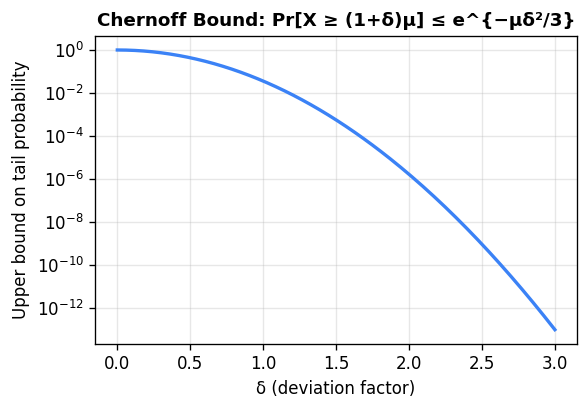
\[ \Pr[X \ge (1+\delta)\mu] \le \left(\frac{e^\delta}{(1+\delta)^{1+\delta}}\right)^\mu. \]\[ \Pr[X \ge (1+\delta)\mu] \le e^{-\mu\delta^2/3}, \qquad \Pr[X \le (1-\delta)\mu] \le e^{-\mu\delta^2/2}. \]For large deviations, if \(R \ge 6\mu\) then \(\Pr[X \ge R] \le 2^{-R}\). Combined: \(\Pr[|X - \mu| \ge \delta\mu] \le 2e^{-\mu\delta^2/3}\).
The same bounds hold by the Hoeffding extension when each \(X_i \in [0,1]\) (not just \(\{0,1\}\)). They also hold when the variables are negatively correlated (intuitively, making one large makes others smaller), since in that case \(\mathbb{E}[e^{t(X+Y)}] \le \mathbb{E}[e^{tX}] \cdot \mathbb{E}[e^{tY}]\). This extension matters for random spanning trees and similar combinatorial objects.
To appreciate the power of Chernoff bounds, revisit the coin-flip example. With \(n\) fair coins and \(\mu = n/2\), \(\Pr[\text{heads} \ge 3n/4] \le e^{-n(1/2)^2/3} = e^{-n/12}\). The probability is exponentially small, compared to the constant \(2/3\) from Markov.
Chernoff bounds also immediately give a clean probability amplification argument. If a BPP algorithm has success probability \(0.6\), then after \(k\) independent repetitions, the expected number of failures is \(0.4k\). The probability that a majority of runs fail equals \(\Pr[\text{failures} \ge k/2]\), and since \(k/2 > (1 + 1/4) \cdot 0.4k\), the Chernoff bound gives \(e^{-\Omega(k)}\). Setting \(k = O(\log n)\) reduces the failure probability to \(1/n^c\) for any desired constant \(c\).
Part III: Hashing, Balls and Bins, and Streaming
The probabilistic ideas we have developed find a natural home in the analysis of hash functions and data structures. The balls-and-bins model captures the essential randomness in hashing, and streaming algorithms exploit this randomness to process massive data sets with tiny working memory.
Balls and Bins
Throw \(m\) balls uniformly and independently into \(n\) bins. The expected load of any fixed bin is \(m/n\). When \(m = n\), the expected number of empty bins is \(n \cdot (1 - 1/n)^n \approx n/e \approx 0.37n\). The question of when all bins are occupied is exactly the coupon collector problem: we need \(m \approx n \ln n\) balls.
This is less than \(1/2\) when \(m \approx \sqrt{2n \ln 2}\). So roughly \(\sqrt{n}\) people suffice for a better-than-even chance of a shared birthday (with \(n = 365\), this is about 23 people).
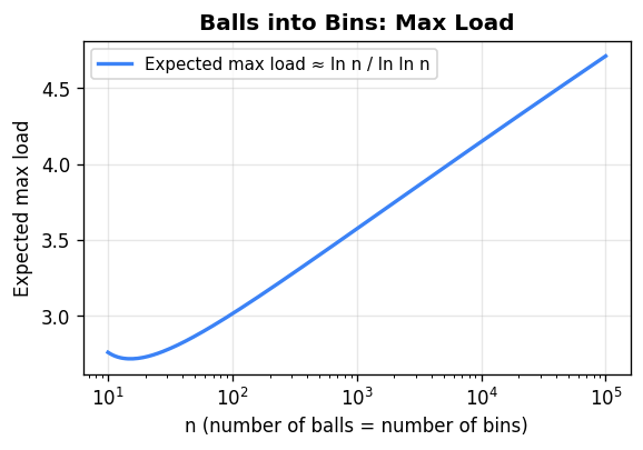
Maximum load. When \(n\) balls land in \(n\) bins, the heaviest bin receives \(\Theta(\ln n / \ln \ln n)\) balls with high probability. For the upper bound, fix a bin and let \(k = \lceil e \ln n / \ln \ln n \rceil\). By the union bound over all possible sets of \(k\) balls hitting this bin, and summing over all \(n\) bins, the probability any bin receives \(\ge k\) balls is at most \(n \cdot \binom{n}{k}(1/n)^k \le n \cdot (e/k)^k = 1/n\) for this choice of \(k\).
Power of two choices. A striking improvement comes from a small modification: for each ball, choose two bins uniformly at random and place the ball in the less loaded one (breaking ties arbitrarily). Under this rule, the maximum load drops to \(O(\ln \ln n)\) — an exponential improvement over the single-choice maximum of \(\Theta(\ln n / \ln \ln n)\). The intuition is that even a small amount of choice essentially eliminates heavily loaded bins from contention.
Poisson approximation. The Binomial\((n, p)\) distribution converges to Poisson\((np)\) as \(n \to \infty\) with \(np = \lambda\) fixed. In the balls and bins setting with \(m\) balls and \(n\) bins, each bin’s load is approximately Poisson\((m/n)\). A useful feature of the Poisson distribution is that the loads of different bins become approximately independent (even though in reality they are negatively correlated), which simplifies analyses. For Poisson\((\lambda)\), standard Chernoff-type bounds give \(\Pr[X \ge k] \le (e\lambda/k)^k e^{-\lambda}\).
Hash Tables and Hash Functions
The goal of a hash table is to maintain a dynamic set \(S \subseteq U\) with \(|S| = n\) and \(|U| = m \gg n\), supporting lookup, insertion, and deletion in \(O(1)\) expected time using \(O(n)\) space. A hash function \(h : U \to \{0, \ldots, n-1\}\) maps universe elements to table positions; collisions are resolved by chaining (each table position holds a linked list).
A truly random hash function — one where all elements hash uniformly and independently — would guarantee optimal performance but requires \(O(m \log n)\) bits to store, which is far too much. The key insight of universal hashing is that much weaker randomness suffices for good performance.
Bloom Filters
A Bloom filter is a space-efficient probabilistic data structure for set membership queries, tolerating false positives. It consists of a bit array \(T\) of length \(\ell\), initially all zeros, together with \(k\) independent hash functions \(h_1, \ldots, h_k : U \to \{0, \ldots, \ell - 1\}\).
To insert \(x\), set \(T[h_i(x)] = 1\) for all \(i\). To query \(x\), return YES if \(T[h_i(x)] = 1\) for all \(i\). There are no false negatives; any inserted element is always found. False positives occur when all \(k\) hash positions of a non-member happen to be set by other elements.
\[ \left(1 - e^{-kn/\ell}\right)^k. \]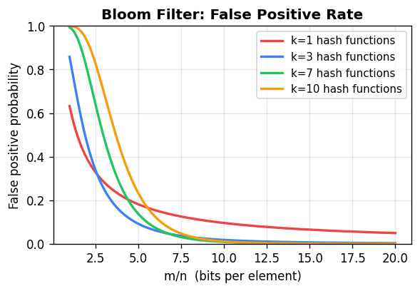 To minimize this over \(k\) for fixed \(\ell/n\), one finds the optimal \(k = (\ell/n) \ln 2\), giving a false positive rate of approximately \((0.6185)^{\ell/n}\). With \(\ell = 8n\) bits per element and \(k = 5\) or \(6\) hash functions, the false positive rate is around 2%. This is a dramatic improvement over a single hash function, which at the same space budget gives a false positive rate near 11%.
\(k\)-wise Independence
Random variables \(X_1, \ldots, X_n\) are \(k\)-wise independent if any \(k\) of them are mutually independent. Pairwise independence (\(k=2\)) is the most commonly used case and is far cheaper to achieve than full independence.
A simple construction of pairwise independent bits: let \(X_1, X_2 \sim \text{Bernoulli}(1/2)\) be independent, and set \(X_3 = X_1 \oplus X_2\). The three variables are pairwise independent but not 3-wise independent. More generally, from \(b\) mutually independent bits \(X_1, \ldots, X_b\), one can derive \(2^b - 1\) pairwise independent bits by forming \(Y_S = \bigoplus_{i \in S} X_i\) for each non-empty \(S \subseteq [b]\). This exponential expansion of randomness from a small seed is a cornerstone of derandomization.
Pairwise independence suffices for Chebyshev’s inequality: if \(X = \sum X_i\) with \(X_i\) pairwise independent, then \(\text{Var}[X] = \sum \text{Var}[X_i]\) still holds (since cross-covariance terms vanish under pairwise independence), and Chebyshev applies. However, Chernoff-type bounds do not extend to pairwise independence; achieving exponential concentration requires stronger independence.
Universal Hash Function Families
\[ \Pr_{h \in \mathcal{H}}[h(x_i) = y_i \text{ for all } i] = \frac{1}{n^k}. \]A family is \(k\)-universal if for distinct \(x_1, \ldots, x_k\), \(\Pr[h(x_1) = \cdots = h(x_k)] \le 1/n^{k-1}\).
The canonical construction of a strongly 2-universal family uses a prime \(p \ge |U|\) and defines \(h_{a,b}(x) = ax + b \pmod{p}\) for coefficients \(a, b \in \{0, \ldots, p-1\}\). For distinct \(x, x'\) and any target values \(y, y'\), the system \(ax + b \equiv y\) and \(ax' + b \equiv y'\) has a unique solution \((a, b)\) over \(\mathbb{Z}_p\), so \(\Pr[h(x) = y \text{ and } h(x') = y'] = 1/p^2\). The family requires only \(O(\log |U|)\) bits to describe a single hash function.
With a 2-universal family, the expected number of collisions in a table of size \(n\) holding \(m\) elements is at most \(\binom{m}{2}/n\). When \(m = n\), expected collisions are at most \(1/2\), and a lookup takes \(O(1)\) expected time.
Perfect Hashing
For a static set \(S\) with \(|S| = m\), perfect hashing achieves \(O(1\)) worst-case lookup time using \(O(m)\) space. The two-level construction achieves this:
In the first level, hash all \(m\) elements into a table of size \(m\) using a 2-universal function \(h_1\). Let \(c_i\) be the number of elements in bucket \(i\). In the second level, for each bucket \(i\), use a separate table of size \(c_i^2\) with a 2-universal function \(h_{2,i}\) chosen so there are no collisions within the bucket (this succeeds with probability at least \(1/2\) by Markov).
The total space is \(m + \sum_i c_i^2\). Since \(\mathbb{E}[\sum_i c_i^2] = \mathbb{E}[\sum_i c_i + 2\binom{c_i}{2}] = m + 2 \cdot (\text{expected collisions}) \le m + 2\binom{m}{2}/m \le 2m\), the expected total space is \(O(m)\). Repeating level-1 hashing until \(\sum c_i^2 \le 4m\) succeeds after \(O(1)\) expected trials, giving perfect hashing with \(O(m)\) space and \(O(1)\) worst-case lookup.
Data Streaming
In the data streaming model, a sequence of updates \((a_1, l_1), (a_2, l_2), \ldots, (a_T, l_T)\) arrives, where \(a_t \in [m]\) is an element identifier and \(l_t\) is a weight (positive or negative). Let \(x_i = \sum_{j : a_j = i} l_j\) be the final count for element \(i\). The vector \(x \in \mathbb{R}^m\) is the frequency vector. The goal is to answer queries about \(x\) using \(O(\text{polylog}(m, T))\) space — far less than storing \(x\) explicitly.
Heavy Hitters and Count-Min Sketch. An element \(i\) is a \(q\)-heavy hitter if \(x_i \ge q \cdot \|x\|_1\). The Count-Min Sketch uses \(k\) independent hash tables, each of size \(\ell\), with independent 2-universal hash functions \(h_1, \ldots, h_k : [m] \to [\ell]\). For each update \((a_t, l_t)\), add \(l_t\) to position \(h_j(a_t)\) in table \(j\), for all \(j\). To estimate \(x_i\), return \(\min_j \{\text{count}_{j,h_j(i)}\}\).
Since the hash functions are 2-universal, for any fixed \(i\) and table \(j\), the expected contribution of other elements to position \(h_j(i)\) is at most \(\|x\|_1 / \ell\). By Markov’s inequality, the probability that this contribution exceeds \(\varepsilon \|x\|_1\) is at most \(1/(\varepsilon \ell)\). Taking \(k\) independent tables, the probability that all of them overestimate by more than \(\varepsilon \|x\|_1\) is at most \((1/(\varepsilon \ell))^k\). Setting \(\ell = 1/\varepsilon\) and \(k = \log(1/\delta)\) gives a \((1 \pm \varepsilon)\) estimate with failure probability \(\delta\), using \(O(\log(1/\delta)/\varepsilon)\) total counters.
Distinct Elements. The goal is to estimate \(D = |\{a_1, \ldots, a_T\}|\), the number of distinct elements seen. The elegant approach is to hash all elements into \(\{1, \ldots, \ell\}\) using a strongly 2-universal hash function and maintain the \(t = O(1/\varepsilon^2)\) smallest values seen. If \(T_t\) is the \(t\)-th smallest hash value, then \(\hat{D} = t \cdot \ell / T_t\) is an estimator of \(D\). By pairwise independence and Chebyshev’s inequality, \(\hat{D}\) is within a factor \((1 \pm \varepsilon)\) of \(D\) with probability at least \(2/3\). Running \(O(\log(1/\delta))\) independent copies and taking the median boosts the success probability to \(1 - \delta\). Total space is \(O(\varepsilon^{-2} \log m \log(1/\delta))\).
Frequency Moments. Define \(F_p = \sum_{i=1}^m x_i^p\). Note \(F_0\) is the number of distinct elements, \(F_1 = \|x\|_1\) is the total count (trivially maintained), and \(F_2 = \|x\|_2^2\) measures the skewness of the distribution.
The AMS estimator (Alon-Matias-Szegedy) for \(F_2\) works as follows. For each element \(i \in [m]\), draw a Rademacher random variable \(r_i\) with \(\Pr[r_i = +1] = \Pr[r_i = -1] = 1/2\), independently across elements. Maintain the running sum \(Z = \sum_t r_{a_t} l_t = \sum_i r_i x_i\). Output \(\hat{F}_2 = Z^2\).
The estimator is unbiased: \(\mathbb{E}[Z^2] = \sum_i x_i^2 + \sum_{i \ne j} x_i x_j \mathbb{E}[r_i r_j] = \sum_i x_i^2 = F_2\), since \(\mathbb{E}[r_i r_j] = 0\) for \(i \ne j\). A calculation gives \(\text{Var}[Z^2] \le 2F_2^2\). By Chebyshev, maintaining \(k = O(1/\varepsilon^2)\) independent copies and averaging gives a \((1 \pm \varepsilon)\) approximation with probability \(2/3\). The crucial efficiency: 4-wise independent Rademacher variables suffice (not full independence), and a 4-wise independent hash family requires only \(O(\log m)\) bits per function, so the total space is \(O(\varepsilon^{-2} \log m)\).
Part IV: Randomized Graph Algorithms
Karger’s Min-Cut Algorithm
The minimum cut problem asks for a minimum cardinality (or minimum weight) edge set whose removal disconnects a given graph \(G = (V, E)\). Deterministically, we can compute minimum cuts by running maximum flow between all pairs, but this is expensive. Karger’s algorithm gives a strikingly simple randomized approach.
The random contraction algorithm repeatedly picks a uniformly random edge and contracts it (merging its two endpoints into a single vertex, keeping multi-edges, removing self-loops), until only two vertices remain. The edges between those two vertices form the output cut.
Theorem. For any specific minimum cut \(F\) with \(|F| = k\), the probability that the algorithm outputs \(F\) is at least \(2/(n(n-1))\).
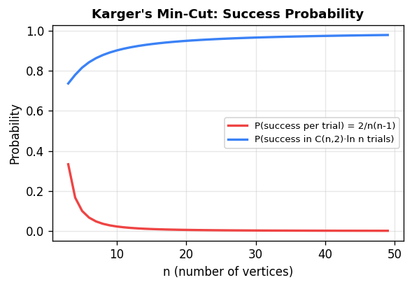
Since success probability is \(\Omega(1/n^2)\), repeating \(cn^2/2\) times and taking the best result yields a minimum cut with probability at least \(1 - (1 - 2/(n(n-1)))^{cn^2/2} \ge 1 - e^{-c}\). The total running time is \(O(n^4)\).
Karger-Stein improves this to \(\tilde{O}(n^2)\) by sharing the early iterations (where failure probability is small) and branching into two independent copies only after the graph shrinks to \(n/\sqrt{2}\) vertices (where failure probability first becomes significant). The recursion \(T(n) = 2T(n/\sqrt{2}) + O(n^2)\) solves to \(T(n) = O(n^2 \log n)\).
A beautiful combinatorial corollary: any undirected graph has at most \(\binom{n}{2}\) distinct minimum cuts. This follows because each minimum cut survives the algorithm with probability at least \(2/(n(n-1))\), and probabilities over disjoint events cannot exceed 1.
Isolating Cuts
A deeper algorithmic idea is to find minimum cuts that isolate individual terminals. Given a terminal set \(R \subseteq V\), the minimum isolating cut for vertex \(v \in R\) is the minimum weight cut \(S_v\) with \(v \in S_v\) and \(R \setminus \{v\} \subseteq V \setminus S_v\). Computing all \(|R|\) such cuts naively requires \(|R|\) max-flow computations, but an elegant structural argument reduces this to \(O(\log |R|)\) max-flow calls.
\[ d_w(A) + d_w(B) \ge d_w(A \cap B) + d_w(A \cup B). \]This follows from the observation that every edge is counted on both sides of the inequality at least as many times as on the right. Submodularity implies that minimum isolating cuts can be made vertex-disjoint by an uncrossing argument: if \(S_u\) and \(S_v\) overlap, we can replace them with \(S_u \cap S_v\) and \(S_u \cup S_v\) (or \(S_u \setminus S_v\) and \(S_v \setminus S_u\)) without increasing cost, and the result is a valid pair of isolating cuts.
The efficient algorithm labels the terminals \(0, 1, \ldots, |R|-1\) in binary. For each bit position \(t \in \{0, \ldots, \lceil \log_2 |R| \rceil\}\), it computes a minimum \(A_t\text{-}B_t\) cut \(C_t\), where \(A_t\) and \(B_t\) are the terminals whose \(t\)-th bit is 0 or 1 respectively. Since no two distinct terminals agree on all bits, the intersection of the cuts \(\{C_t : \text{terminal } v\text{'s bit } t = 0\}\) separates \(v\) from all other terminals. In total, only \(O(\log |R|)\) max-flow computations are needed.
The minimum Steiner cut problem asks for the minimum weight cut \((S, V \setminus S)\) with \(S \cap R \ne \emptyset\) and \((V \setminus S) \cap R \ne \emptyset\). A randomized reduction to max-flow works as follows: if the minimum Steiner cut separates \(k\) terminals from the rest, sample each terminal independently with probability \(1/k\). With probability approximately \(1/e\), exactly one terminal is sampled; conditioning on this, we have reduced to a single-terminal minimum isolating cut. Iterating over \(k = 2^0, 2^1, \ldots\) with \(O(\log n)\) repetitions each gives an \(O(\log^3 n)\) max-flow algorithm for minimum Steiner cut with high probability.
Part V: Approximation Algorithms and Graph Sparsification
The randomized techniques developed so far — contraction, sampling, and Chernoff bounds — combine naturally with linear programming to give approximation algorithms, and with structural properties of cuts to give sparsification.
Randomized Rounding for Congestion Minimization
The congestion minimization problem routes \(k\) source-sink pairs \((s_i, t_i)\) on a graph \(G\), where each pair must be routed along a single path, and the goal is to minimize the maximum number of paths sharing any edge (the congestion).
Write a linear programming relaxation: let \(f^i_P \ge 0\) be the fractional amount of flow for pair \(i\) routed on path \(P\), with \(\sum_P f^i_P = 1\) for each \(i\). The LP congestion on edge \(e\) is \(\sum_i \sum_{P \ni e} f^i_P\). Let \(C^*\) be the LP optimum.
Randomized rounding: independently for each pair \(i\), choose a path \(P\) with probability \(f^i_P\). This is an integral solution.
\[ O\!\left(C^* \cdot \frac{\ln n}{\ln \ln n}\right) \]with probability at least \(1 - 1/n\). This remains the best known approximation ratio for congestion minimization.
Cut Sparsification
\[ (1 - \varepsilon)\, w_G(\delta(S)) \le w_H(\delta(S)) \le (1 + \varepsilon)\, w_G(\delta(S)) \]for every \(S \subseteq V\). The goal is to find \(H\) with far fewer edges than \(G\) while preserving all cut information up to a \((1 \pm \varepsilon)\) factor.
\[ \Pr\!\left[\,|w_H(\delta(S)) - w_G(\delta(S))| > \varepsilon \, w_G(\delta(S))\right] \le 2 n^{-5|\delta_G(S)|/c}. \]To union bound over all \(2^n\) cuts, we use a structural lemma: the number of cuts with at most \(\alpha c\) edges is at most \(n^{2\alpha}\). This follows from the same probabilistic argument as Karger’s min-cut — each such small cut survives the contraction algorithm with probability \(\Omega(n^{-2\alpha})\), and these probabilities must sum to at most 1 over disjoint cuts. Grouping cuts by size and summing the Chernoff failures gives total failure probability at most \(4/n\).
The resulting sparsifier \(H\) has \(O(n \log n / \varepsilon^2)\) edges in expectation, reducible to \(O(n \log n / \varepsilon^2)\) deterministically. Benczúr and Karger extended this to arbitrary graphs — without a minimum cut assumption — by sampling each edge with probability proportional to its strong connectivity, with the same sparsity and approximation guarantee.
Part VI: Dimension Reduction and Compressed Sensing
High-dimensional geometry is expensive: storing and processing point sets in \(\mathbb{R}^d\) costs time and space proportional to \(d\). A remarkable family of random linear maps allows projecting high-dimensional data to much lower dimensions while preserving pairwise distances.
The Johnson-Lindenstrauss Lemma
\[ (1 - \varepsilon)\,\|x_i - x_j\|_2^2 \le \|A(x_i) - A(x_j)\|_2^2 \le (1+\varepsilon)\,\|x_i - x_j\|_2^2. \]The construction is \(A(x) = (1/\sqrt{k})\, M x\), where \(M\) is a \(k \times d\) matrix with i.i.d. \(\mathcal{N}(0,1)\) entries. To analyze this, fix a unit vector \(u \in \mathbb{R}^d\) and examine \(\|Au\|_2^2 = (1/k) \sum_{j=1}^k (M_j \cdot u)^2\), where \(M_j\) is the \(j\)-th row of \(M\). Since \(u\) is a unit vector, each \(M_j \cdot u \sim \mathcal{N}(0,1)\), so \(\|Au\|_2^2\) has a scaled chi-squared distribution with \(k\) degrees of freedom.
\[ \Pr\!\left[\,\|Au\|_2^2 > 1 + \varepsilon\right] \le e^{-k\varepsilon^2/8}, \qquad \Pr\!\left[\,\|Au\|_2^2 < 1 - \varepsilon\right] \le e^{-k\varepsilon^2/8}. \]Setting \(k = O(\varepsilon^{-2} \log(1/\delta))\) ensures failure probability at most \(\delta\) for any fixed unit vector \(u\). With \(\delta = 1/n^2\), a union bound over all \(\binom{n}{2}\) pairs guarantees the JL property simultaneously for all pairs. An identical analysis works for random \(\pm 1\) matrices (Achlioptas’s construction), which are more computationally efficient.
Applications of JL are numerous: approximate nearest neighbor search (project to low dimension, then search), approximate matrix multiplication, and fast algorithms for numerical linear algebra.
Compressed Sensing and the Restricted Isometry Property
Compressed sensing asks: if an unknown signal \(x \in \mathbb{R}^n\) is \(s\)-sparse (has at most \(s\) nonzero coordinates), can we recover it from \(k \ll n\) linear measurements \(b = Ax\)?
The obstacle is that \(\ell_0\)-minimization (finding the sparsest vector consistent with the measurements) is NP-hard in general. The breakthrough insight is that if the sensing matrix \(A\) satisfies a geometric property called the Restricted Isometry Property (RIP), then \(\ell_0\)-minimization is equivalent to the tractable \(\ell_1\)-minimization \(\min \{\|x\|_1 : Ax = b\}\).
\[ (1 - \varepsilon)\,\|x\|_2^2 \le \|Ax\|_2^2 \le (1 + \varepsilon)\,\|x\|_2^2. \]Theorem. If \(A\) is \((3s, \varepsilon)\)-RIP with \(\varepsilon < 1/9\), then the unique \(s\)-sparse solution to \(Ax = b\) is the unique solution to \(\min\{\|x\|_1 : Ax = b\}\).
Proving this theorem involves a careful \(\ell_1\)/\(\ell_2\) inequality. Let \(x^*\) be the true \(s\)-sparse signal and \(x\) be the \(\ell_1\) minimizer. Let \(\Delta = x - x^*\) and let \(S\) be the support of \(x^*\). Since \(x\) minimizes \(\ell_1\) and \(\|x\|_1 \le \|x^*\|_1\), we get \(\|\Delta_S\|_1 \ge \|\Delta_{\bar{S}}\|_1\) (the perturbation outside the support cannot help). Decompose \(\Delta_{\bar{S}}\) into blocks \(B_1, B_2, \ldots\) of size \(s\) sorted by magnitude. A geometric argument using this sorted structure shows \(\sum_{j \ge 2} \|\Delta_{B_j}\|_2 \le \|\Delta_S\|_2 / \sqrt{s}\). Applying RIP to \(\Delta_{S \cup B_1}\) and using the bound on the tail, one concludes \(\|\Delta\|_2 = 0\), so \(x = x^*\).
For the RIP construction: take \(A = (1/\sqrt{k}) M\) where \(M\) is \(k \times n\) with i.i.d. \(\mathcal{N}(0,1)\) entries. Fix any subset \(T\) of \(s\) coordinates. The restriction of \(A\) to columns in \(T\) is itself a Gaussian embedding, and by JL-type arguments, it preserves lengths of all vectors with support in \(T\) up to \((1 \pm \varepsilon)\). An \(\varepsilon\)-net of the unit sphere in \(s\) dimensions has at most \((4/\varepsilon)^s\) points. Union bounding over the net and all \(\binom{n}{s}\) subsets, with \(k = O(s \log n / \varepsilon^2)\) measurements, \(A\) is \((s, \varepsilon)\)-RIP with high probability.
Part VII: The Probabilistic Method
The probabilistic method is a non-constructive proof technique: to show that an object with a certain combinatorial property exists, define a probability space over objects and show the desired property holds with positive probability. Since probability cannot be positive and yet no object exist, the object must exist.
First Moment Arguments
If \(X\) is an integer-valued random variable with \(\mathbb{E}[X] > 0\), then \(\Pr[X \ge 1] > 0\), and by definition there exists an outcome where \(X \ge 1\). Equivalently, if \(\mathbb{E}[X] < 1\) for a non-negative integer-valued \(X\), then \(\Pr[X = 0] > 0\).
Independent sets. Any graph \(G\) on \(n\) vertices with \(m \ge n/2\) edges has an independent set of size at least \(n^2/(4m)\). Include each vertex independently with probability \(p = n/(2m)\). Remove one endpoint from each remaining edge. Expected remaining vertices: \(np - mp^2 = n \cdot n/(2m) - m \cdot n^2/(4m^2) = n^2/(4m)\). So some choice of \(p\) realizes this expected value.
\[ \Pr[\text{some monochromatic } K_k] \le \binom{n}{k} \cdot 2^{1-\binom{k}{2}}. \]This is less than 1 when \(k \ge 2\log_2 n\) (approximately), so a valid 2-coloring exists. Deterministic constructions avoiding \(K_{O(\log n)}\) remain an outstanding open problem.
High girth, high chromatic number. For any \(k\) and \(\ell\), there exist graphs with chromatic number greater than \(k\) and girth (shortest cycle length) greater than \(\ell\). Consider \(G(n, p)\) with \(p = n^{\varepsilon - 1}\) for \(\varepsilon < 1/\ell\). The expected number of short cycles is \(o(n)\), and the expected maximum independent set has size \(O(n^{1-\varepsilon} \log n)\). Deleting one vertex per short cycle removes at most \(n/2\) vertices (with high probability), leaving a graph with girth \(> \ell\) and chromatic number \(\Omega(n^\varepsilon / \log n)\), which is large for large \(n\). This deletion method — constructing the desired object by removing the bad configurations from a random one — is a key technique.
Threshold Phenomena in Random Graphs
The random graph \(G(n,p)\) includes each of the \(\binom{n}{2}\) edges independently with probability \(p\). Many graph properties exhibit a sharp threshold: there is a function \(f(n)\) such that the property almost surely fails when \(p = o(f(n))\) and almost surely holds when \(p = \omega(f(n))\).
The giant component emerges at \(p = 1/n\). For \(p < (1-\varepsilon)/n\), all components have size \(O(\log n)\). For \(p > (1+\varepsilon)/n\), a unique giant component of size \(\Omega(\varepsilon^2 n)\) appears, and all other components have size \(O(\log n)\). This phase transition, discovered by Erdős and Rényi, is one of the landmark results in probabilistic combinatorics.
With the probabilistic toolkit now assembled, we turn to one of the most powerful tools for probabilistic existence arguments in combinatorics and algorithms: the Lovász Local Lemma.
Part VIII: The Lovász Local Lemma
Statement and Motivation
We want to show that a collection of “bad” events \(E_1, \ldots, E_m\) can simultaneously be avoided: \(\Pr[\bigcap_i \bar{E}_i] > 0\). The union bound handles this when \(\sum_i \Pr[E_i] < 1\), but it is useless when there are many events each with nontrivial probability. At the other extreme, if the events are mutually independent, we need only \(\Pr[E_i] < 1\) for each \(i\).
The Lovász Local Lemma (LLL) handles the intermediate case, where events are nearly independent — each event depends on few others. Define the dependency graph by connecting \(i\) and \(j\) with an edge if \(E_i\) is not mutually independent of \(E_j\).
Theorem (Symmetric LLL). Suppose each event \(E_i\) has probability at most \(p\), and each event depends on at most \(d\) others. If \(4dp \le 1\), then \(\Pr[\bigcap_i \bar{E}_i] > 0\).
\[ \Pr[E_i] \le x_i \prod_{j \in \Gamma(i)} (1 - x_j), \]where \(\Gamma(i)\) is the neighborhood of \(i\) in the dependency graph. Then \(\Pr[\bigcap_i \bar{E}_i] \ge \prod_i (1 - x_i) > 0\).
The condition \(4dp \le 1\) in the symmetric version corresponds to setting \(x_i = 1/(2d)\) in the asymmetric version. The LLL applies a local version of the union bound: each event is unlikely enough relative to the events it directly influences.
Proof
\[ \Pr\!\left[E_k \;\middle|\; \bigcap_{i \in S} \bar{E}_i\right] \le x_k. \]\[ \Pr\!\left[E_k \;\middle|\; \bigcap_{i \in S} \bar{E}_i\right] = \frac{\Pr\!\left[E_k \cap \bigcap_{i \in S_1} \bar{E}_i \;\middle|\; \bigcap_{j \in S_2} \bar{E}_j\right]}{\Pr\!\left[\bigcap_{i \in S_1} \bar{E}_i \;\middle|\; \bigcap_{j \in S_2} \bar{E}_j\right]}. \]Since \(E_k\) is mutually independent of \(\{\bar{E}_j : j \in S_2\}\), the numerator is at most \(\Pr[E_k] \le x_k \prod_{j \in \Gamma(k)}(1-x_j)\). For the denominator, iterating the inductive hypothesis gives \(\Pr[\bigcap_{i \in S_1} \bar{E}_i \mid \bigcap_{j \in S_2} \bar{E}_j] \ge \prod_{i \in S_1}(1-x_i) \ge \prod_{j \in \Gamma(k)}(1-x_j)\). Dividing yields the claim.
Applications
\(k\)-SAT. If each clause in a \(k\)-CNF formula contains \(k\) literals and each variable appears in at most \(2^k/(4k)\) clauses, a satisfying assignment exists. Each clause is violated with probability \(2^{-k}\) under a random assignment. Each clause shares a variable with at most \(k \cdot 2^k/(4k) - 1 < 2^{k-2}\) other clauses. The symmetric LLL applies since \(4 \cdot 2^{k-2} \cdot 2^{-k} = 1\).
Graph coloring. If each vertex \(v\) has at least \(8r\) available colors and each color appears in at most \(r\) neighbors of \(v\), then a proper coloring using the available colors exists. The bad event \(B_{e,c}\) is that edge \(e = \{u,v\}\) is monochromatic with color \(c\). We have \(\Pr[B_{e,c}] \le 1/(8r)^2\). Each bad event \(B_{e,c}\) can conflict with at most \(2 \cdot 8r \cdot r = 16r^2\) other bad events. Setting \(x = 1/(64r^2)\) in the asymmetric LLL: \(4 \cdot 16r^2 \cdot (1/(64r^2)) = 1\), and the condition is satisfied.
Palette sparsification. A striking application: in a graph of maximum degree \(\Delta\), give each vertex \(K = 24\Delta\) colors and let each vertex sample an \(L(v)\)-element palette by choosing \(O(\sqrt{\log n})\) colors uniformly at random. The LLL (combined with Chernoff bounds to control the “c-degree” of each color in each neighborhood) implies that a proper coloring exists using only the sampled palettes, with high probability. This reduces the number of colors per vertex from \(K\) to \(O(\sqrt{\log n})\) while maintaining colorability.
Moser’s Constructive Algorithm
The original LLL proof is existential. In 2009, Robin Moser gave a simple, efficient algorithm to find a satisfying assignment for \(k\)-SAT formulas satisfying the LLL condition:
Algorithm: Solve-SAT
Input: k-CNF formula with clauses C_1, ..., C_m
---
1. Initialize: assign each variable uniformly at random
2. While some clause C_i is unsatisfied:
   Call Fix(C_i)

Fix(C):
1. Resample all variables in C uniformly at random
2. For each clause D sharing a variable with C, in order of index:
   If D is unsatisfied: call Fix(D)
---
Output: current assignment
The algorithm is analyzed by a compression argument. Suppose the algorithm runs for \(t\) steps without terminating. Encode the execution as follows: the initial random assignment uses \(n\) bits. The execution tree (which Fix calls which) can be encoded in \(O(t \log m)\) bits. But crucially, given the execution tree and the final assignment, we can reconstruct all random bits used: each time Fix\((C)\) is called, it resamples \(k\) bits, but we know these bits must have been the unique assignment that violates \(C\) (since Fix was called precisely because \(C\) was violated). So we get \(k\) bits for free per Fix call. This compression saves approximately \(t(k - \log m - O(1))\) bits out of the total \(n + tk\) bits used. Since random bits cannot be compressed, \(t(k - \log m - O(1)) = O(n)\), giving \(t = O(nm/(k - \log m))\). Under the symmetric LLL condition \(d \le 2^{k-3}\), we have \(k - \log d \ge 3\), so the algorithm terminates in \(O(m \log m)\) expected steps.
Part IX: Martingales and Discrepancy
Martingales and Azuma-Hoeffding
The Chernoff bound applies to sums of independent random variables. For sums of dependent variables — where the dependence is structured — martingale theory provides analogous concentration results.
A sequence of random variables \(X_0, X_1, \ldots\) is a martingale with respect to a sequence \(Y_1, Y_2, \ldots\) if:
- \(X_i\) is determined by \(Y_1, \ldots, Y_i\) (it is measurable with respect to the first \(i\) observations),
- \(\mathbb{E}[|X_i|] < \infty\), and
- \(\mathbb{E}[X_{i+1} \mid Y_1, \ldots, Y_i] = X_i\).
The martingale property says the process has no drift: the expected next value equals the current value. A key consequence is \(\mathbb{E}[X_n] = \mathbb{E}[X_0]\) for all \(n\).
The most versatile construction is the Doob martingale. Given a random variable \(Z = f(Y_1, \ldots, Y_n)\) and the sequence of observations \(Y_1, \ldots, Y_n\), define \(X_i = \mathbb{E}[Z \mid Y_1, \ldots, Y_i]\). The sequence \(X_0 = \mathbb{E}[Z], X_1, \ldots, X_n = Z\) is a martingale. The process represents the successive refinement of our estimate of \(Z\) as observations are revealed one by one.
\[ \Pr\!\left[|X_n - X_0| \ge \lambda\right] \le 2 \exp\!\left(\frac{-\lambda^2}{2 \sum_i c_i^2}\right). \]The proof parallels the Chernoff bound proof. Write \(D_i = X_i - X_{i-1}\) for the martingale differences, so \(|D_i| \le c_i\) and \(\mathbb{E}[D_i \mid Y_1,\ldots,Y_{i-1}] = 0\). By the convexity of the exponential function, \(\mathbb{E}[e^{tD_i} \mid Y_1, \ldots, Y_{i-1}] \le e^{t^2 c_i^2/2}\). Multiplying over all \(i\) by the tower property of expectation gives \(\mathbb{E}[e^{t(X_n - X_0)}] \le e^{t^2 \sum c_i^2 / 2}\). Markov then gives the result, and one optimizes over \(t\).
Method of Bounded Differences
\[ \Pr\!\left[|f(Y) - \mathbb{E}[f(Y)]| > \lambda\right] \le 2 \exp\!\left(\frac{-\lambda^2}{2\sum_i c_i^2}\right). \]A canonical application is the chromatic number of a random graph. For \(G \sim G(n, p)\), the chromatic number \(\chi(G)\) changes by at most 1 when any single edge is added or removed (since adding an edge can increase \(\chi\) by at most 1, and removing one cannot increase it at all; the relevant parameter is vertex exposure, each changing \(\chi\) by at most 1). So \(\Pr[|\chi(G) - \mathbb{E}[\chi(G)]| > \lambda] \le 2e^{-\lambda^2/(2n)}\). This gives strong concentration of \(\chi(G)\) even though its exact value is unknown.
Discrepancy Minimization
\[ \text{disc}(\chi) = \max_{j \in [m]} \left|\sum_{i \in S_j} \chi(i)\right|. \]A random signing gives discrepancy \(O(\sqrt{n \log m})\) with high probability (by Chernoff applied to each set, and union bound over all \(m\) sets). The question is whether one can do better.
Spencer’s theorem (1985) says one can always do much better: there exists a signing with discrepancy at most \(K\sqrt{n}\) when \(m = n\), for a universal constant \(K\). The striking statement “six standard deviations suffice” refers to \(K = 6\).
The Lovett-Meka algorithm (2012) provides a constructive proof via a random walk. The idea is partial coloring: instead of finding a complete \(\pm 1\) signing directly, find a vector \(\chi \in [-1, 1]^n\) such that at least \(n/2\) coordinates are near \(\pm 1\) (say, have absolute value \(\ge 1 - \delta\)), while the discrepancy constraints \(|\langle \chi, \mathbf{1}_{S_j}\rangle| \le c_j\) are all satisfied. Recurse on the remaining coordinates.
The algorithm maintains the current partial coloring \(\chi_t\) and takes a random walk within the feasible polytope. At each step, it computes the subspace \(V_t\) orthogonal to all nearly-tight constraints (both variable constraints \(|\chi_i| \le 1\) and discrepancy constraints \(|\langle \chi, \mathbf{1}_{S_j}\rangle| \le c_j\)), then updates \(\chi_{t+1} = \chi_t + \varepsilon u_t\) where \(u_t\) is a random Gaussian vector in \(V_t\).
The analysis proceeds in two parts. First, a martingale concentration argument shows that few discrepancy constraints become tight: setting \(c_j = 8\sqrt{n \log(m/n)}\), the assumption \(\sum_j e^{-c_j^2/16} \le n/16\) is satisfied, and the number of tight discrepancy constraints grows slowly. Second, a dimension argument shows that the dimension of \(V_t\) remains large, so the walk continues to make progress on variable constraints: after \(T = K_1 / \varepsilon^2\) steps, at least \(0.65n\) coordinates are near \(\pm 1\). Setting \(c_j = O(\sqrt{n \log(m/n)})\) for all \(j\) achieves discrepancy \(O(\sqrt{n \log(m/n)})\), matching Spencer’s bound.
Part X: Spectral Sparsification
Cut sparsification preserves all cut values. Spectral sparsification is a strictly stronger guarantee: the sparse graph \(H\) approximates the graph \(G\) as a quadratic form, meaning the Laplacians satisfy \((1-\varepsilon)L_G \preceq L_H \preceq (1+\varepsilon)L_G\) in the positive semidefinite order. This implies cut approximation (since cuts correspond to \(\{0,1\}\) quadratic forms), but also approximates more general properties like eigenvalues, effective resistances, and random walk behavior.
Graph Laplacians
\[ x^T L_G x = \sum_{\{u,v\} \in E} w_{uv}(x_u - x_v)^2 \ge 0, \]so \(L_G\) is positive semidefinite (PSD). Writing \(b_e\) for the vector with \(\sqrt{w_e}\) at endpoint \(u\), \(-\sqrt{w_e}\) at endpoint \(v\), and 0 elsewhere, we have \(L_G = \sum_{e \in E} b_e b_e^T\), an explicit PSD decomposition.
A graph \(H\) is a \((1\pm\varepsilon)\)-spectral approximator of \(G\) if \((1-\varepsilon)L_G \preceq L_H \preceq (1+\varepsilon)L_G\), meaning for every vector \(x\): \((1-\varepsilon) x^T L_G x \le x^T L_H x \le (1+\varepsilon) x^T L_G x\).
The Sampling Framework and Effective Resistance
The Spielman-Srivastava theorem says every graph has a spectral sparsifier with \(O(n \log n / \varepsilon^2)\) edges. The construction reduces to a linear algebraic problem. Define the vectors \(v_e = L_G^{\dagger/2} b_e\), where \(L_G^\dagger\) is the pseudoinverse of \(L_G\). These satisfy \(\sum_{e \in E} v_e v_e^T = I\) (the identity on the image of \(L_G\)).
Sampling edge \(e\) with probability \(p_e\) and weight \(w_e / p_e\) corresponds to forming a random matrix \(\sum_e s_e v_e v_e^T\) where \(s_e = 1/p_e\) with probability \(p_e\) and 0 otherwise. The spectral approximation condition becomes: \((1-\varepsilon)I \preceq \sum_e s_e v_e v_e^T \preceq (1+\varepsilon)I\).
\[ \|v_e\|_2^2 = b_e^T L_G^\dagger b_e = R_{\text{eff}}(u, v), \]the effective resistance of edge \(e = \{u,v\}\) in the electrical network where each edge has resistance \(1/w_e\). Cut edges have effective resistance 1 (they carry all current) and must always be sampled. Edges in dense subgraphs have small effective resistance and can be sampled rarely. This connection between spectral sparsification and electrical networks is deep and fruitful.
Matrix Chernoff Bound
The analysis of the random sampling procedure uses a matrix analogue of the scalar Chernoff bound.
\[ \Pr\!\left[\lambda_{\max}\!\left(\sum_i X_i\right) \ge (1+\varepsilon)\mu_{\max}\right] \le n\, e^{-\varepsilon^2 \mu_{\max}/(3R)}, \]\[ \Pr\!\left[\lambda_{\min}\!\left(\sum_i X_i\right) \le (1-\varepsilon)\mu_{\min}\right] \le n\, e^{-\varepsilon^2 \mu_{\min}/(2R)}. \]Applying this to the spectral sparsification problem: we sample each vector independently \(C = 6\log n / \varepsilon^2\) times. In each trial, the matrix \(X_{e,t} = v_e v_e^T / (C p_e)\) with probability \(p_e\) and 0 otherwise has \(\mathbb{E}[X_{e,t}] = v_e v_e^T / C\), and \(X_{e,t} \preceq (1/C) I\) since \(v_e v_e^T \le \|v_e\|_2^2 I = p_e I\). Summing, \(\sum_{e,t} \mathbb{E}[X_{e,t}] = I\), so \(\mu_{\min} = \mu_{\max} = 1\) and \(R = 1/C\). The failure probability from Tropp’s bound is at most \(n e^{-\varepsilon^2 C / 3} = n e^{-2\log n} = 1/n\).
The total number of sampled edges is \(C \cdot \sum_e p_e = C \cdot \text{tr}(I) = Cn = O(n \log n / \varepsilon^2)\). A near-linear time algorithm for estimating all effective resistances (using Laplacian solvers) gives a near-linear time sparsification algorithm overall. The Batson-Spielman-Srivastava theorem shows the optimal bound of \(O(n/\varepsilon^2)\) edges is achievable, even deterministically, though the algorithm is more involved.
Part XI: Numerical Linear Algebra
The tools of randomization apply not just to combinatorial problems but to the core problems of numerical linear algebra. The key insight is that many problems become easier when the data matrix is first compressed by a random projection.
Subspace Embeddings and Least Squares
The least squares problem asks, given \(A \in \mathbb{R}^{n \times d}\) with \(n \gg d\) and \(b \in \mathbb{R}^n\), to find \(x^* = \arg\min_x \|Ax - b\|_2\). The exact solution costs \(O(nd^2)\) time. The goal is to find an approximate solution \(\hat{x}\) with \(\|A\hat{x} - b\|_2 \le (1+\varepsilon)\|Ax^* - b\|_2\) in faster time.
A subspace embedding for the column space of \([A \mid b]\) is a matrix \(S \in \mathbb{R}^{k \times n}\) with \(k \ll n\) satisfying \((1-\varepsilon)\|Ax - b\|_2 \le \|S(Ax-b)\|_2 \le (1+\varepsilon)\|Ax-b\|_2\) for all \(x\) simultaneously. If such \(S\) exists, solving \(\min_x \|SAx - Sb\|_2\) in \(O(kd^2)\) time gives the desired approximation.
Three constructions achieve different speed-space tradeoffs:
A Gaussian embedding uses \(S = (1/\sqrt{k})M\) with \(M\) a \(k \times n\) i.i.d. \(\mathcal{N}(0,1)\) matrix, \(k = O(d/\varepsilon^2)\). Applying \(S\) to \(A\) costs \(O(nd \cdot k) = O(nd^2/\varepsilon^2)\) — slower than the direct method.
CountSketch uses a \(k \times n\) matrix where each column has exactly one nonzero entry \(\pm 1\) in a random row. Equivalently, hash each coordinate of a vector to a random bucket and add it (with random sign). With \(k = O(d^2/\varepsilon^2)\), CountSketch is a subspace embedding, and applying it costs \(O(\text{nnz}(A))\) time — optimal for sparse \(A\).
The Subsampled Randomized Hadamard Transform (SRHT) uses \(S = (1/\sqrt{k})RHD\), where \(D\) is a random diagonal \(\pm 1\) matrix, \(H\) is the normalized Hadamard transform (computable in \(O(n \log n)\)), and \(R\) randomly samples \(k\) rows. With \(k = O(d\log d/\varepsilon^2)\), SRHT is a subspace embedding and applying it to \(A\) costs \(O(nd\log n)\) — the fastest known bound, though larger than CountSketch’s \(O(\text{nnz}(A))\) for sparse matrices.
Laplacian Solvers
Solving a linear system \(Lx = b\) where \(L\) is a graph Laplacian is a fundamental algorithmic problem, arising in electrical flow, random walks, max-flow, and many other settings. Direct methods cost \(O(n^\omega) \approx O(n^{2.37})\). The Spielman-Teng theorem (2004) gives a nearly linear time algorithm.
The key technique is to use a spectral sparsifier as a preconditioner. If \(\tilde{L}\) is a \((1\pm\varepsilon)\)-spectral approximation to \(L\), then solving \(Lx = b\) via the preconditioned conjugate gradient method with preconditioner \(\tilde{L}\) converges in \(O(1/\sqrt{\varepsilon})\) iterations — but each iteration requires solving \(\tilde{L} z = r\). By applying this recursively — solving the sparsified system with an even sparser preconditioner, and so on — one obtains a hierarchical solver that runs in \(O(n\,\text{polylog}\,n)\) time. Laplacian solvers have become a central tool in modern algorithm design, enabling near-linear time algorithms for network flow, random spanning trees, and graph problems.
Part XII: Random Walks and Electrical Networks
Random Walks on Graphs
A random walk on a graph \(G = (V, E)\) starts at some vertex and at each step moves to a uniformly random neighbor. The central questions are:
- Stationary distribution: what fraction of time is spent at each vertex in the long run?
- Hitting time \(h_{uv}\): expected number of steps to first reach \(v\) starting from \(u\).
- Cover time \(C(G)\): expected steps to visit every vertex, starting from the worst initial vertex.
- Mixing time \(\tau(\varepsilon)\): time until the distribution over vertices is within total variation \(\varepsilon\) of the stationary distribution.
Formally, a random walk on \(G\) is a Markov chain with state space \(V\) and transition matrix \(P_{uv} = 1/\deg(u)\) if \(\{u,v\} \in E\), and 0 otherwise. The chain is irreducible (any vertex is reachable from any other) and, for non-bipartite graphs, aperiodic. The stationary distribution \(\pi\) satisfies \(\pi P = \pi\) and is given by \(\pi(v) = \deg(v)/(2|E|)\).
Hitting Time and Cover Time
A fundamental result bounds the hitting time in terms of the graph’s edge count.
Theorem. For any vertices \(u, v\) in a graph with \(|E| = m\), \(h_{uv} \le 2m(n-1)\).
This follows from the structural bound on the commute time \(C_{uv} = h_{uv} + h_{vu}\), which we compute below via electrical networks.
\[ C(G) \le \sum_{\{u,v\} \in T} C_{uv} \le 2m(n-1) \le n^3. \]The path graph \(P_n\) achieves \(C(P_n) = \Theta(n^2)\), which is tight for the bound \(2m(n-1)\) with \(m = n-1\).
Electrical Networks and Effective Resistance
\[ R_{\text{eff}}(u,v) = \phi(u) - \phi(v) = b_{uv}^T L^\dagger b_{uv} = (e_u - e_v)^T L^\dagger (e_u - e_v). \]Theorem (Commute Time Formula). \(C_{uv} = h_{uv} + h_{vu} = 2m \cdot R_{\text{eff}}(u,v)\).
The proof uses the optional stopping theorem applied to the voltage function. Consider the function \(f(w) = c_u \phi(w)\) where \(\phi\) is the voltage when unit current enters at \(u\) and exits at \(v\), and \(c_u = \phi(u) - \phi(v) = R_{\text{eff}}\). One verifies that \(f(X_t) - t \cdot (\text{const})\) is a martingale, and applying optional stopping at the first hitting time of \(v\) recovers the formula.
Since each edge has \(R_{\text{eff}}(u,v) \le 1\) (by the parallel law — adding paths only reduces resistance, and the direct edge gives resistance \(1/w_{uv} \le 1\) for unit weights), we get \(C_{uv} \le 2m\) for adjacent vertices.
The spectral interpretation: the normalized Laplacian \(\mathcal{L} = D^{-1/2}(D-A)D^{-1/2}\) has eigenvalues \(0 = \lambda_1 \le \lambda_2 \le \cdots \le \lambda_n \le 2\). The spectral gap \(\lambda_2\) controls mixing: \(\tau(\varepsilon) = O(\log(n/\varepsilon)/\lambda_2)\). The effective resistance between vertices \(u\) and \(v\) can be expressed in terms of the eigenvectors of \(\mathcal{L}\), revealing a deep connection between the spectral and electrical views of graphs.
Part XIII: Mixing Time, MCMC, and Coupling
Conductance and the Lovász-Simonovits Method
\[ \Phi = \min_{S : \pi(S) \le 1/2} \frac{\sum_{u \in S, v \notin S} \pi(u) P_{uv}}{\pi(S)}. \]For the simple random walk on an unweighted graph, this simplifies to \(\Phi = \min_{S} w(\delta(S))/(2m \cdot \pi(S))\). Conductance measures how quickly probability flows out of the worst bottleneck set.
Cheeger’s inequality relates conductance to the spectral gap: \(\lambda_2/2 \le \Phi \le \sqrt{2\lambda_2}\). The upper bound says high conductance implies a large spectral gap; the lower bound says even moderate conductance suffices for a nontrivial gap. As a consequence, for the \(d\)-dimensional hypercube (where \(\Phi = 1/d\)), the mixing time is \(\Theta(d \log d)\).
The Lovász-Simonovits curve method gives a direct proof of mixing from conductance without computing eigenvalues. The idea is to track the “profile” of the distribution as the walk progresses and show that each step brings the profile closer to uniform. If the conductance is \(\Phi_0\), then after \(T = O(\Phi_0^{-2} \log(n/\varepsilon))\) steps, the total variation distance to stationarity is at most \(\varepsilon\).
Markov Chain Monte Carlo
Many important distributions are hard to sample from directly but can be specified by a local structure. Markov Chain Monte Carlo (MCMC) constructs a Markov chain whose stationary distribution is the target \(\pi\), then runs the chain until it mixes.
Metropolis-Hastings is the general template. Given a proposal distribution \(Q(x, \cdot)\), a proposed move from \(x\) to \(y\) is accepted with probability \(\min(1, \pi(y)Q(y,x)/(\pi(x)Q(x,y)))\). The chain satisfies detailed balance: \(\pi(x)P(x,y) = \pi(y)P(y,x)\), which implies \(\pi\) is the stationary distribution. The freedom to choose \(Q\) allows designing chains that explore the state space efficiently.
Glauber dynamics for graph coloring with \(k\) colors (where \(k > 2\Delta\) and \(\Delta\) is the maximum degree):
Algorithm: Glauber Dynamics
State: a proper k-coloring chi of G
---
1. Repeat:
   a. Pick a uniformly random vertex v
   b. Let A(v) = {colors not used by any neighbor of v}
   c. Color v uniformly at random from A(v)
---
Output: samples from the uniform distribution over proper k-colorings
When \(k > 2\Delta\), every step has \(|A(v)| \ge k - \Delta > \Delta\), ensuring the chain is well-defined. The chain is ergodic: any coloring is reachable from any other. For \(k > 2\Delta\), the mixing time is \(O(n \log n)\) — the chain mixes in nearly linear time.
Counting via Sampling
MCMC samplers enable approximate counting. To count the number of proper \(k\)-colorings of \(G\), use a self-reducibility argument: start with a complete graph \(K_n\) (where the count is \(k!/(k-n)!\) if \(k \ge n\), easily computed) and successively delete edges until we reach \(G\). At each edge deletion \(e = \{u,v\}\), the ratio of colorings before and after is estimated by the fraction of colorings in the current graph where \(u\) and \(v\) have different colors — which equals \(\Pr[\chi(u) \ne \chi(v)]\) under a random coloring of the current graph, estimable by running the MCMC sampler. Multiplying together all \(|E|\) ratios gives an approximation to the total count.
Coupling
\[ \|p - q\|_{\text{TV}} \le \Pr[X \ne Y], \]and equality is achieved by the “maximal coupling.” To bound the mixing time, construct a coupling of two copies of the Markov chain — one started from an arbitrary initial state \(x\), the other from the stationary distribution \(\pi\) — and show the two copies coalesce (hit the same state) in time \(\tau\) with high probability. By the coupling lemma, the total variation distance at time \(\tau\) is at most \(\Pr[\text{not coalesced by time } \tau]\).
Example (lazy random walk on the path). Couple two walkers \((X_t, Y_t)\) on the path \(\{1, \ldots, n\}\) so they always move in the same direction. The difference \(|X_t - Y_t|\) performs a lazy random walk on \(\{0, 1, \ldots, n-1\}\), which hits 0 in expected time \(O(n^2)\). So the mixing time of the lazy random walk on the path is \(O(n^2)\).
Coupling for Glauber dynamics. Couple two chains \((\chi_t, \chi'_t)\) that differ in exactly one vertex’s color. At each step, both chains update the same vertex \(v\). If \(v\) is not the disagreeing vertex, the same random color is chosen for both (using the same random variable), keeping the disagreement localized. If \(v\) is the disagreeing vertex, both chains recolor it from their respective available color sets; one can couple so the disagreement is eliminated unless the available sets differ significantly. When \(k > 2\Delta\), the expected number of disagreements decreases each step, and the Hamming distance \(d_t = |\{v : \chi_t(v) \ne \chi'_t(v)\}|\) is a supermartingale. Azuma-Hoeffding then gives \(O(n \log n)\) mixing.
Part XIV: Algebraic Methods
Algebraic tools — polynomials, linear algebra over finite fields — provide a powerful suite of randomized algorithms for problems that seem purely combinatorial.
Polynomial Identity Testing and Schwartz-Zippel
\[ \Pr[p(r_1, \ldots, r_n) = 0] \le \frac{d}{|S|}. \]The proof is by induction on \(n\). Write \(p = \sum_{i=0}^{d_1} x_1^i q_i(x_2, \ldots, x_n)\), where \(d_1 \le d\) is the degree of \(p\) in \(x_1\) and \(q_{d_1} \not\equiv 0\). By induction, \(\Pr[q_{d_1}(r_2,\ldots,r_n) = 0] \le (d - d_1)/|S|\). Conditioned on \(q_{d_1} \ne 0\), the polynomial \(p(x_1, r_2, \ldots, r_n)\) is a nonzero univariate of degree \(d_1\), which has at most \(d_1\) roots; so \(\Pr[p(r_1, \ldots, r_n) = 0 \mid q_{d_1} \ne 0] \le d_1/|S|\). Combining gives \(d/|S|\).
The immediate application is polynomial identity testing (PIT): to check if two multivariate polynomials \(p\) and \(q\) are identical, evaluate \(p - q\) at a random point from a large set \(S\) with \(|S| = 2d\). If \(p \ne q\), then \(p - q\) is a nonzero polynomial of degree at most \(d\), and the test rejects with probability at least \(1/2\). Repeat \(O(\log(1/\delta))\) times for failure probability \(\delta\). The key advantage: the polynomial need not be written explicitly — it suffices to evaluate it at a point, and the evaluation may be much faster than any explicit expansion.
Perfect Matching in Bipartite Graphs
\[ \det(T(G)) \ne 0 \text{ as a polynomial} \iff G \text{ has a perfect matching}. \]This is because the determinant expands as \(\sum_\sigma \text{sgn}(\sigma) \prod_i x_{i,\sigma(i)}\), and each term corresponds to a perfect matching. If any matching exists, its term cannot cancel (since the variables \(x_{ij}\) are distinct).
To test for a perfect matching: substitute random integers from \(\{1, \ldots, 2n\}\) for each variable \(x_{ij}\), and evaluate the determinant modulo a prime \(p \approx n^2\). By Schwartz-Zippel, \(\Pr[\det = 0 \mid G\text{ has a matching}] \le n/(2n) = 1/2\). This gives a randomized \(O(n^\omega)\) algorithm, where \(\omega < 2.37\) is the matrix multiplication exponent.
Finding the matching itself (not just detecting it) can be done by trying to delete edges and checking whether the determinant drops to zero. Alternatively, Gaussian elimination on the Tutte matrix over a finite field reveals the matching structure.
Parallel Computation
The algebraic approach naturally parallelizes. Computing the rank of a matrix modulo a prime can be done in \(O(\log^2 n)\) parallel time with polynomially many processors (the complexity class \(\mathbf{NC}^2\)). Since detecting a perfect matching reduces to rank computation, perfect matching is in randomized \(\mathbf{NC}\) (the class \(\mathbf{RNC}\)). A deterministic \(\mathbf{NC}\) algorithm for perfect matching remains a major open problem.
Network Coding
Consider a directed graph with one source \(s\) and multiple sinks \(t_1, \ldots, t_k\). Each edge carries one symbol per time step from a field \(\mathbb{F}_q\). The goal is to multicast: transmit all \(n\) source symbols simultaneously to all sinks, at the maximum possible rate (the information-theoretic limit is the minimum \(s\)-to-any-sink cut value).
A linear network code assigns to each outgoing edge at each node a linear combination (over \(\mathbb{F}_q\)) of the signals on its incoming edges. The remarkable result of Ahlswede, Cai, Li, and Yeung (2000) is that linear codes can achieve the min-cut bound for multicast — there is no need for complex coding strategies.
Random linear network coding makes this constructive and efficient: each node assigns coefficients for its outgoing edges uniformly at random over \(\mathbb{F}_q\). Let \(M_i\) be the \(n \times n\) “transfer matrix” from source to sink \(t_i\), whose entries are polynomials in the coding coefficients. If a valid linear network code exists, then \(\det(M_i) \ne 0\) as a polynomial (the code achieves rate \(n\) iff \(M_i\) is invertible). By Schwartz-Zippel, the probability that random coefficients make any \(\det(M_i) = 0\) is at most \(kn/q\). Choosing \(q \ge 2kn\) ensures success with probability at least \(1/2\).
Interactive Proofs
An interactive proof system for a language \(L\) is a protocol between an all-powerful prover \(P\) and a polynomial-time verifier \(V\). The verifier must accept all \(x \in L\) and reject all \(x \notin L\) (with high probability). The class \(\mathbf{IP}\) contains all languages with interactive proofs.
The sum-check protocol is the foundational interactive proof technique. Given a multilinear polynomial \(p\) of degree \(d\) in \(n\) variables over a prime field \(\mathbb{F}\), the protocol verifies the claim \(\sum_{x \in \{0,1\}^n} p(x) = v\). In round \(i\), the prover sends the univariate polynomial \(s_i(x_i) = \sum_{x_{i+1},\ldots,x_n \in \{0,1\}} p(r_1,\ldots,r_{i-1},x_i,x_{i+1},\ldots,x_n)\) and the verifier checks consistency with the previous round’s value, then picks a random challenge \(r_i\). After \(n\) rounds, the verifier evaluates \(p(r_1,\ldots,r_n)\) directly. Soundness: if \(v\) is wrong, by Schwartz-Zippel, the probability the verifier is fooled in any given round is at most \(d/|\mathbb{F}|\). Union bound over \(n\) rounds gives failure probability at most \(nd/|\mathbb{F}|\).
The theorem \(\mathbf{IP} = \mathbf{PSPACE}\) (Shamir 1990) says every PSPACE computation has an interactive proof. The key application of sum-check: counting satisfying assignments of a quantified Boolean formula (which is PSPACE-complete) reduces to evaluating a sum of an arithmetic circuit over the Boolean hypercube.
Graph Non-Isomorphism (GNI) illustrates the power of interaction. To prove two graphs \(G_0\) and \(G_1\) are non-isomorphic: the verifier picks \(b \in \{0,1\}\) uniformly at random, randomly permutes \(G_b\), and sends the permuted graph \(H\) to the prover. An honest prover (who can distinguish non-isomorphic graphs) returns \(b\) correctly. A cheating prover (who cannot distinguish the graphs) can only guess \(b\) correctly with probability \(1/2\). Repeating \(k\) times reduces the cheating probability to \(2^{-k}\). Since GNI has no obvious \(\mathbf{NP}\) proof (a proof of non-isomorphism would require checking all \(n!\) permutations), this interactive proof is genuinely more powerful than an NP witness.
Part XV: Property Testing
What is Property Testing?
A property tester for a property \(\mathcal{P}\) distinguishes two cases with bounded error: the input has property \(\mathcal{P}\), or the input is \(\varepsilon\)-far from having \(\mathcal{P}\) (meaning we must change at least an \(\varepsilon\) fraction of the input to make it satisfy \(\mathcal{P}\)). The goal is sublinear query complexity — testing without reading the entire input. This is achievable because we do not need to handle the intermediate case (inputs that are slightly far from \(\mathcal{P}\)).
With the algebraic and probabilistic tools assembled, we can now tackle testing problems for sequences and distributions.
Testing Sortedness
Given an array \(x[1], \ldots, x[n]\) of distinct values, we want to decide whether \(x\) is sorted, or must change at least \(\varepsilon n\) entries to make it sorted. Naively, checking every pair of consecutive entries requires \(O(n)\) queries. Can we do better?
The elegant approach uses binary search. An element \(x[i]\) is searchable if running binary search for \(x[i]\) in the array \(x\) terminates at position \(i\). In a sorted array, every element is searchable. If \(x\) is \(\varepsilon\)-far from sorted, at least \(\varepsilon n\) elements are non-searchable.
Algorithm: Test-Sortedness
Input: array x[1..n], parameter eps
---
Repeat O(log(1/delta) / eps) times:
   Pick a uniformly random index i in {1, ..., n}
   Run binary search for x[i] in x
   If binary search does not land at i: return "not sorted"
Return "sorted"
---
Output: decision
Each iteration uses \(O(\log n)\) queries. If the array is sorted, binary search always succeeds, so the algorithm correctly returns “sorted.” If the array is \(\varepsilon\)-far from sorted, there are at least \(\varepsilon n\) non-searchable elements, and a random index finds one with probability at least \(\varepsilon\). After \(O(\log(1/\delta)/\varepsilon)\) trials, the failure probability is at most \(\delta\). Total query complexity: \(O(\varepsilon^{-1} \log n \log(1/\delta))\) — dramatically sublinear.
Testing Distributions
Given i.i.d. samples from an unknown distribution \(P\) over \([n]\), we want to test whether \(P\) equals a specified distribution \(Q\), or \(\|P - Q\|_1 \ge \varepsilon\). For the special case of uniformity testing (where \(Q = U_n\, \), the uniform distribution), the key statistic is the collision probability \(\|P\|_2^2 = \sum_i p_i^2\). For \(P = U_n\), this equals \(1/n\). If \(\|P - U_n\|_1 \ge \varepsilon\), then by Cauchy-Schwarz, \(\|P - U_n\|_2^2 \ge \varepsilon^2/n\), so \(\|P\|_2^2 \ge 1/n + \varepsilon^2/n\).
The collision estimator \(Z = \binom{m}{2}^{-1}\sum_{i The same framework generalizes to testing against an arbitrary reference distribution \(Q\) using the chi-squared statistic \(Z(Q) = \sum_i (N_i - mq_i)^2/(mq_i) - N_i/(mq_i)\), where \(N_i\) is the observed count for symbol \(i\). This is an unbiased estimator of \(n(\|P/Q\|_2^2 - 1)\), and similar Chebyshev analysis gives sample complexity \(O(\sqrt{n}/\varepsilon^2)\). Testing monotone distributions. A distribution \(P\) over \([n]\) is monotone if \(p_1 \ge p_2 \ge \cdots \ge p_n\). Testing whether \(P\) is monotone or \(\varepsilon\)-far from monotone requires first learning \(P\) approximately under chi-squared distance, then running a uniformity tester against the learned approximation. The sample complexity is \(O(n\log n/\varepsilon^4 + \sqrt{n}/\varepsilon^2)\), dominated by the learning phase. Naive anonymization — removing names or other obvious identifiers — provides much weaker protection than expected. Three cautionary examples illustrate the problem. In 2006, Netflix released anonymized movie ratings for a machine learning competition. Narayanan and Shmatikiv re-identified individual users by cross-referencing the anonymized ratings with public IMDB reviews: knowing only a handful of obscure movies a person rated and approximately when they were rated was sufficient to uniquely identify that person in the Netflix database. In 2008, Homer et al. showed that genome-wide association study (GWAS) summary statistics — aggregate allele frequencies, not individual records — could nonetheless reveal whether a specific individual participated in the study, using chi-squared statistics. The NIH consequently stopped releasing certain aggregate genomic statistics. In 1997, Latanya Sweeney demonstrated that Massachusetts medical records, purportedly anonymous, could be re-identified by combining them with publicly available voter registration records (ZIP code, date of birth, and sex). This triple uniquely identifies 87% of Americans, even though each field alone seems innocuous. These failures share a common thread: the attacker combines the released data with external information. Any meaningful privacy framework must be robust to arbitrary auxiliary information. Even releasing only aggregate statistics can be dangerous. A stark formalization: suppose a mechanism \(M\) answers every subset-sum query \(q_S(x) = |x \cap S|\) on a database \(x \in \{0,1\}^n\) with additive error at most \(\alpha\). Dinur and Nissim proved: Theorem (Dinur-Nissim). If a mechanism answers all \(2^n\) subset-sum queries with error at most \(\alpha < 1/4\), then one can reconstruct \(x' \in \{0,1\}^n\) with normalized Hamming distance \(d_H(x, x')/(n) \le 4\alpha\) — essentially recovering the entire database. The attack uses only \(O(n)\) random queries. Each query \(q_S\) is answered with value \(a_S = q_S(x) + \eta_S\) where \(|\eta_S| \le \alpha\). Consider the optimization problem: find \(x' \in \{0,1\}^n\) minimizing \(\sum_S (q_S(x') - a_S)^2\). This least-squares problem concentrates around the true database \(x\), and a counting argument (using the Paley-Zygmund inequality, a reverse Markov bound) shows the reconstruction is accurate with constant probability. The implication is stark: any mechanism that answers many queries accurately enough necessarily reconstructs the database. The question of how many queries one can safely answer motivates differential privacy. Randomized response (Warner, 1965) provides local privacy for binary data: each person independently reports their true bit \(b_i\) with probability \((1+\varepsilon)/2\) and flips it with probability \((1-\varepsilon)/2\). An observer can estimate the population mean with error \(O(1/(\varepsilon\sqrt{n}))\) but cannot determine any individual’s response with confidence. Central differential privacy (Dwork, McSherry, Nissim, Smith, 2006) gives a stronger formal guarantee: the entire database is processed by a trusted curator who adds noise before releasing results. With \(\delta = 0\), we say \(M\) is \(\varepsilon\)-differentially private. The interpretation: an adversary who observes the output cannot determine whether any single individual participated in the database. This holds even with arbitrary auxiliary information, since the privacy guarantee is about the mechanism’s output distribution, not the adversary’s knowledge. The parameter \(\varepsilon\) controls the privacy-accuracy tradeoff. Values \(\varepsilon \le 0.1\) give strong privacy; \(\varepsilon \approx 1\) is often considered reasonable in practice. The \(\delta\) term accounts for low-probability catastrophic events; \(\delta\) should be cryptographically small (much smaller than \(1/n\)). The Laplace mechanism outputs \(M(x) = f(x) + (Z_1, \ldots, Z_k)\) where \(Z_i \sim \text{Lap}(\Delta(f)/\varepsilon)\) are i.i.d. Laplace random variables with scale \(\Delta/\varepsilon\). Theorem. The Laplace mechanism is \(\varepsilon\)-differentially private. For mean estimation: \(f(x) = (1/n)\sum_i b_i\) with \(b_i \in \{0,1\}\) has sensitivity \(\Delta = 1/n\). The Laplace mechanism outputs \(f(x) + \text{Lap}(1/(n\varepsilon))\) with error \(O(1/(n\varepsilon))\) — quadratically better than randomized response’s \(O(1/(\varepsilon\sqrt{n}))\) — but requires a trusted curator. Differential privacy enjoys several pleasant closure properties. Post-processing: if \(M\) is \((\varepsilon, \delta)\)-DP and \(f\) is any (possibly randomized) function, then \(f(M(x))\) is \((\varepsilon, \delta)\)-DP. Analyzing private data cannot worsen privacy. Group privacy: if \(M\) is \((\varepsilon, 0)\)-DP and databases \(x\) and \(x'\) differ in \(k\) records, then \(\Pr[M(x) \in S] \le e^{k\varepsilon} \Pr[M(x') \in S]\). Privacy degrades gracefully with the size of the group. Basic composition: \(k\) mechanisms each \((\varepsilon, 0)\)-DP compose to \((k\varepsilon, 0)\)-DP. Privacy costs add linearly. Advanced composition: \(k\) mechanisms each \((\varepsilon, 0)\)-DP compose to \((\varepsilon', k\varepsilon(e^\varepsilon - 1) + \delta')\)-DP where \(\varepsilon' = \sqrt{2k\ln(1/\delta')} \cdot \varepsilon\). The savings — a \(\sqrt{k}\) factor in \(\varepsilon\) compared to basic composition — are essential for releasing many statistics while maintaining a reasonable privacy budget. These composition properties, combined with the Laplace mechanism and its variants (Gaussian mechanism, exponential mechanism), form a rich toolkit for designing differentially private algorithms for a wide range of statistical tasks: histograms, regression, principal component analysis, synthetic data generation, and machine learning. The field continues to mature rapidly, bridging theoretical foundations with practical deployment in major technology systems.Part XVI: Data Privacy and Differential Privacy
Failures of Anonymization
The Dinur-Nissim Attack
Differential Privacy
The Laplace Mechanism
\[
\Delta(f) = \max_{x, y \text{ neighboring}} \|f(x) - f(y)\|_1.
\]Composition and Post-Processing