MATH 138: Calculus 2 for Honours Mathematics
Estimated study time: 52 minutes
Table of contents
Chapter 1: Integration
1.1 Areas Under Curves
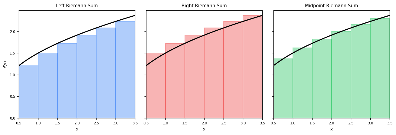
The fundamental problem motivating integration is finding the area under a curve. Using the Method of Exhaustion (dating back to Archimedes and Eudoxus), we approximate the area under \(f(x) = x^2\) on \([0,1]\) with rectangles. As the number of rectangles \(n \to \infty\), both the right-hand estimate \(R_n\) and left-hand estimate \(L_n\) converge to \(\frac{1}{3}\).
A parallel motivation comes from the relationship between displacement and velocity: the displacement equals the area under the velocity curve, since \(s = v \Delta t\) for constant velocity generalizes via Riemann sums.
1.2 Riemann Sums and the Definite Integral
Definition (Riemann Sum). Given a bounded function \(f\) on \([a,b]\), a partition \(P\): \(a = t_0 < t_1 < \cdots < t_n = b\), and points \(c_i \in [t_{i-1}, t_i]\), a Riemann sum for \(f\) with respect to \(P\) is
\[ S = \sum_{i=1}^n f(c_i)\,\Delta t_i. \]Definition (Regular \(n\)-Partition). Given an interval \([a,b]\) and \(n \in \mathbb{N}\), the regular \(n\)-partition of \([a,b]\) is the partition where each subinterval has the same length \(\Delta t_i = \frac{b-a}{n}\), with \(t_i = a + i\cdot\frac{b-a}{n}\).
Definition (Right-hand Riemann Sum). The right-hand Riemann sum for \(f\) with respect to \(P\) is obtained by choosing \(c_i = t_i\):
\[ R = \sum_{i=1}^n f(t_i)\,\Delta t_i. \]For the regular \(n\)-partition, \(R_n = \sum_{i=1}^n f\!\left(a + i\frac{b-a}{n}\right)\frac{b-a}{n}\).
Definition (Left-hand Riemann Sum). The left-hand Riemann sum is obtained by choosing \(c_i = t_{i-1}\):
\[ L = \sum_{i=1}^n f(t_{i-1})\,\Delta t_i. \]Definition (Definite Integral). A bounded function \(f\) is integrable on \([a,b]\) if there exists a unique number \(I \in \mathbb{R}\) such that whenever \(\{P_n\}\) is a sequence of partitions with \(\lim_{n\to\infty}\|P_n\| = 0\) and \(\{S_n\}\) is any associated sequence of Riemann sums, we have \(\lim_{n\to\infty} S_n = I\). We write
\[ I = \int_a^b f(t)\,dt. \]Theorem 1 (Integrability Theorem for Continuous Functions). Let \(f\) be continuous on \([a,b]\). Then \(f\) is integrable on \([a,b]\). Moreover,
\[ \int_a^b f(t)\,dt = \lim_{n\to\infty} R_n = \lim_{n\to\infty} L_n \]where \(R_n\) and \(L_n\) are the right- and left-hand Riemann sums for the regular \(n\)-partition.
This theorem also holds if \(f\) is bounded and has finitely many discontinuities on \([a,b]\).
1.3 Properties of the Definite Integral
Theorem 2 (Properties of Integrals). Assume \(f\) and \(g\) are integrable on \([a,b]\). Then:
(i) \(\int_a^b c\,f(t)\,dt = c\int_a^b f(t)\,dt\) for any \(c \in \mathbb{R}\).
(ii) \(\int_a^b (f+g)(t)\,dt = \int_a^b f(t)\,dt + \int_a^b g(t)\,dt\).
(iii) If \(m \le f(t) \le M\) for all \(t \in [a,b]\), then \(m(b-a) \le \int_a^b f(t)\,dt \le M(b-a)\).
(iv) If \(0 \le f(t)\) on \([a,b]\), then \(0 \le \int_a^b f(t)\,dt\).
(v) If \(g(t) \le f(t)\) on \([a,b]\), then \(\int_a^b g(t)\,dt \le \int_a^b f(t)\,dt\).
(vi) \(|f|\) is integrable on \([a,b]\) and \(\left|\int_a^b f(t)\,dt\right| \le \int_a^b |f(t)|\,dt\).
1.3.1 Additional Properties
Definition (Identical Limits of Integration). Let \(f(t)\) be defined at \(t = a\). Then \(\int_a^a f(t)\,dt = 0\).
Definition (Switching the Limits). If \(f\) is integrable on \([a,b]\) with \(a < b\), then \(\int_a^b f(t)\,dt = -\int_b^a f(t)\,dt\).
Theorem 3 (Integrals over Subintervals). If \(f\) is integrable on an interval \(I\) containing \(a\), \(b\), and \(c\), then
\[ \int_a^b f(t)\,dt = \int_a^c f(t)\,dt + \int_c^b f(t)\,dt. \]1.3.2 Geometric Interpretation
If \(f(x) \ge 0\) on \([a,b]\), then \(\int_a^b f(x)\,dx\) equals the area under the graph. If \(f\) changes sign, the integral equals the area above the \(x\)-axis minus the area below it.
1.4 The Average Value of a Function
Definition (Average Value). If \(f\) is continuous on \([a,b]\), the average value of \(f\) on \([a,b]\) is
\[ \frac{1}{b-a}\int_a^b f(t)\,dt. \]Theorem 4 (Mean Value Theorem for Integrals). If \(f\) is continuous on \([a,b]\), then there exists \(c \in [a,b]\) such that
\[ f(c) = \frac{1}{b-a}\int_a^b f(t)\,dt. \]1.5 The Fundamental Theorem of Calculus (Part 1)
The integral function \(G(x) = \int_a^x f(t)\,dt\) computes the accumulated area under \(f\) starting from \(a\). The rate of change of this area is precisely \(f(x)\).
Theorem 5 (Fundamental Theorem of Calculus, Part 1). Assume \(f\) is continuous on an open interval \(I\) containing \(a\). Let \(G(x) = \int_a^x f(t)\,dt\). Then \(G\) is differentiable at each \(x \in I\) and
\[ G'(x) = \frac{d}{dx}\int_a^x f(t)\,dt = f(x). \]Theorem 6 (Extended FTC). If \(f\) is continuous and \(g\), \(h\) are differentiable, and \(H(x) = \int_{g(x)}^{h(x)} f(t)\,dt\), then
\[ H'(x) = f(h(x))\,h'(x) - f(g(x))\,g'(x). \]1.6 The Fundamental Theorem of Calculus (Part 2)
1.6.1 Antiderivatives
Definition (Antiderivative). Given a function \(f\), an antiderivative is a function \(F\) such that \(F'(x) = f(x)\). If \(F\) is one antiderivative, then all antiderivatives have the form \(G(x) = F(x) + C\).
The indefinite integral \(\int f(x)\,dx\) denotes the family of all antiderivatives.
Theorem 7 (Power Rule for Antiderivatives). If \(\alpha \ne -1\), then
\[ \int x^\alpha\,dx = \frac{x^{\alpha+1}}{\alpha+1} + C. \]1.6.2 Evaluating Definite Integrals
Theorem 8 (Fundamental Theorem of Calculus, Part 2). If \(f\) is continuous and \(F\) is any antiderivative of \(f\), then
\[ \int_a^b f(t)\,dt = F(b) - F(a). \]1.7 Change of Variables
Theorem 9 (Change of Variables). If \(g'(x)\) is continuous on \([a,b]\) and \(f(u)\) is continuous on \(g([a,b])\), then
\[ \int_{x=a}^{x=b} f(g(x))\,g'(x)\,dx = \int_{u=g(a)}^{u=g(b)} f(u)\,du. \]For indefinite integrals, one substitutes \(u = g(x)\), \(du = g'(x)\,dx\), evaluates \(\int f(u)\,du\), and replaces \(u\) by \(g(x)\).
Chapter 2: Techniques of Integration
2.1 Inverse Trigonometric Substitutions
There are three main classes of inverse trig substitutions:
| Integrand form | Substitution | Identity used |
|---|---|---|
| \(\sqrt{a^2 - b^2x^2}\) | \(bx = a\sin(u)\) | \(\sin^2+\cos^2=1\) |
| \(\sqrt{a^2 + b^2x^2}\) | \(bx = a\tan(u)\) | \(\sec^2-1=\tan^2\) |
| \(\sqrt{b^2x^2 - a^2}\) | \(bx = a\sec(u)\) | \(\sec^2-1=\tan^2\) |
For example, using \(x = \sin(u)\) one can show \(\int_{-1}^{1}\sqrt{1-x^2}\,dx = \frac{\pi}{2}\).
2.2 Integration by Parts
Definition (Integration by Parts Formula).
\[ \int f(x)\,g'(x)\,dx = f(x)\,g(x) - \int f'(x)\,g(x)\,dx. \]Theorem 1 (Integration by Parts for Definite Integrals). If \(f'\) and \(g'\) are continuous on an interval containing \(a\) and \(b\), then
\[ \int_a^b f(x)\,g'(x)\,dx = f(x)\,g(x)\Big|_a^b - \int_a^b f'(x)\,g(x)\,dx. \]Integration by Parts is suited for integrals of the types \(\int x^n\cos x\,dx\), \(\int x^n\sin x\,dx\), \(\int x^n e^x\,dx\), \(\int e^x\cos x\,dx\), \(\int e^x\sin x\,dx\), and integrals like \(\int\arctan(x)\,dx\) or \(\int\ln(x)\,dx\) (writing the integrand as \(1 \cdot f(x)\)).
2.3 Partial Fractions
Definition (Type I Partial Fraction Decomposition). If \(f(x) = \frac{p(x)}{q(x)}\) where \(\deg(p) < \deg(q) = k\) and \(q(x) = a(x-a_1)(x-a_2)\cdots(x-a_k)\) with distinct roots, then
\[ f(x) = \frac{1}{a}\left[\frac{A_1}{x-a_1} + \frac{A_2}{x-a_2} + \cdots + \frac{A_k}{x-a_k}\right]. \]Theorem 2 (Integration of Type I Partial Fractions). Under the conditions above,
\[ \int f(x)\,dx = \frac{1}{a}[A_1\ln|x-a_1| + A_2\ln|x-a_2| + \cdots + A_k\ln|x-a_k|] + C. \]Definition (Type II Partial Fraction Decomposition). When \(q(x)\) has repeated roots \(q(x) = a(x-a_1)^{m_1}\cdots(x-a_l)^{m_l}\), each factor \((x-a_j)^{m_j}\) contributes terms \(\frac{A_{j,1}}{x-a_j} + \frac{A_{j,2}}{(x-a_j)^2} + \cdots + \frac{A_{j,m_j}}{(x-a_j)^{m_j}}\).
Definition (Type III Partial Fraction Decomposition). When \(q(x)\) contains an irreducible quadratic factor \(x^2+bx+c\) with multiplicity \(m\), it contributes terms of the form \(\frac{B_1x+C_1}{x^2+bx+c} + \cdots + \frac{B_mx+C_m}{(x^2+bx+c)^m}\).
2.4 Improper Integrals
Definition (Type I Improper Integral).
\(\int_a^\infty f(x)\,dx\) converges if \(\lim_{b\to\infty}\int_a^b f(x)\,dx\) exists.
\(\int_{-\infty}^a f(x)\,dx\) converges if \(\lim_{b\to -\infty}\int_b^a f(x)\,dx\) exists.
\(\int_{-\infty}^{\infty} f(x)\,dx\) converges if both \(\int_{-\infty}^c f(x)\,dx\) and \(\int_c^{\infty} f(x)\,dx\) converge for some \(c\).
Theorem 3 (\(p\)-Test for Type I Improper Integrals). The integral \(\int_1^\infty \frac{1}{x^p}\,dx\) converges if and only if \(p > 1\). When \(p > 1\), \(\int_1^\infty \frac{1}{x^p}\,dx = \frac{1}{p-1}\).
Theorem 4 (Properties of Type I Improper Integrals). If \(\int_a^\infty f(x)\,dx\) and \(\int_a^\infty g(x)\,dx\) both converge, then:
\(\int_a^\infty cf(x)\,dx = c\int_a^\infty f(x)\,dx\).
\(\int_a^\infty (f+g)(x)\,dx = \int_a^\infty f(x)\,dx + \int_a^\infty g(x)\,dx\).
If \(f(x) \le g(x)\) for \(x \ge a\), then \(\int_a^\infty f(x)\,dx \le \int_a^\infty g(x)\,dx\).
If \(a < c < \infty\), then \(\int_c^\infty f(x)\,dx\) converges and \(\int_a^\infty f(x)\,dx = \int_a^c f(x)\,dx + \int_c^\infty f(x)\,dx\).
Theorem 5 (Monotone Convergence Theorem for Functions). If \(f\) is non-decreasing on \([a,\infty)\):
If \(\{f(x) \mid x \in [a,\infty)\}\) is bounded above, then \(\lim_{x\to\infty}f(x) = \text{lub}(\{f(x)\})\).
If not bounded above, then \(\lim_{x\to\infty}f(x) = \infty\).
Theorem 6 (Comparison Test for Type I Improper Integrals). Suppose \(0 \le g(x) \le f(x)\) for all \(x \ge a\) and both are continuous on \([a,\infty)\).
If \(\int_a^\infty f(x)\,dx\) converges, then \(\int_a^\infty g(x)\,dx\) converges.
If \(\int_a^\infty g(x)\,dx\) diverges, then \(\int_a^\infty f(x)\,dx\) diverges.
Definition (Absolute Convergence for Improper Integrals). The integral \(\int_a^\infty f(x)\,dx\) converges absolutely if \(\int_a^\infty |f(x)|\,dx\) converges.
Theorem 7 (Absolute Convergence Theorem for Improper Integrals). If \(\int_a^\infty |f(x)|\,dx\) converges, then \(\int_a^\infty f(x)\,dx\) converges. In particular, if \(0 \le |f(x)| \le g(x)\) and \(\int_a^\infty g(x)\,dx\) converges, then \(\int_a^\infty f(x)\,dx\) converges.
2.4.3 The Gamma Function
Definition (Gamma Function). For \(x \in \mathbb{R}\), define \(\Gamma(x) = \int_0^\infty t^{x-1}e^{-t}\,dt\).
Integration by parts yields the recurrence \(\Gamma(x+1) = x\,\Gamma(x)\). Since \(\Gamma(1) = 1\), induction gives \(\Gamma(n) = (n-1)!\) for \(n \in \mathbb{N}\).
2.4.4 Type II Improper Integrals
Definition (Type II Improper Integral).
If \(f\) has a vertical asymptote at \(x = a\), then \(\int_a^b f(x)\,dx = \lim_{t\to a^+}\int_t^b f(x)\,dx\).
If \(f\) has a vertical asymptote at \(x = b\), then \(\int_a^b f(x)\,dx = \lim_{t\to b^-}\int_a^t f(x)\,dx\).
Theorem 8 (\(p\)-Test for Type II Improper Integrals). The integral \(\int_0^1 \frac{1}{x^p}\,dx\) converges if and only if \(p < 1\). When \(p < 1\), \(\int_0^1 \frac{1}{x^p}\,dx = \frac{1}{1-p}\).
Chapter 3: Applications of Integration
3.1 Areas Between Curves
If \(f\) and \(g\) are continuous on \([a,b]\), the area of the region between their graphs is
\[ A = \int_a^b |g(t) - f(t)|\,dt. \]When \(f(t) \le g(t)\) on \([a,b]\), this simplifies to \(\int_a^b (g(t)-f(t))\,dt\). When the curves cross, one must split the integral at each crossing point.
3.2 Volumes of Revolution: Disk Method
If \(f\) is continuous on \([a,b]\) with \(f(x) \ge 0\), the volume obtained by rotating the region under \(f\) around the \(x\)-axis is
\[ V = \int_a^b \pi\,[f(x)]^2\,dx. \]More generally, if \(0 \le f(x) \le g(x)\), rotating the region between \(f\) and \(g\) gives
\[ V = \int_a^b \pi\left[(g(x))^2 - (f(x))^2\right]dx. \]For example, the volume of a sphere of radius \(r\) is derived by rotating \(f(x) = \sqrt{r^2-x^2}\), yielding \(V = \frac{4}{3}\pi r^3\).
3.3 Volumes of Revolution: Shell Method
If \(a \ge 0\) and \(f(x) \le g(x)\) on \([a,b]\), the volume obtained by rotating the region between \(f\) and \(g\) around the \(y\)-axis is
\[ V = \int_a^b 2\pi x\,(g(x)-f(x))\,dx. \]3.4 Arc Length
If \(f\) is continuously differentiable on \([a,b]\), the arc length of its graph is
\[ S = \int_a^b \sqrt{1 + (f'(x))^2}\,dx. \]Chapter 4: Differential Equations
4.1 Introduction to Differential Equations
Definition (Differential Equation). A differential equation is an equation \(F(x, y, y', y'', \ldots, y^{(n)}) = 0\). A solution is a function \(\varphi\) satisfying this equation. The highest derivative order is the order of the DE.
4.2 Separable Differential Equations
Definition (Separable DE). A first-order DE is separable if it can be written as \(y' = f(x)\,g(y)\).
Definition (Equilibrium Solution). If \(g(y_0) = 0\), then the constant function \(\varphi(x) = y_0\) is a constant (equilibrium) solution to \(y' = f(x)\,g(y)\).
To solve a separable DE: (1) identify \(f(x)\) and \(g(y)\); (2) find equilibrium solutions where \(g(y_0)=0\); (3) separate variables: \(\int \frac{1}{g(y)}\,dy = \int f(x)\,dx\); (4) solve for \(y\) explicitly.
4.3 First-Order Linear Differential Equations
Definition (First-Order Linear DE). A first-order DE is linear if it can be written as \(y' = f(x)\,y + g(x)\).
Theorem 1 (Solving FOLDEs). The solutions to \(y' = f(x)\,y + g(x)\) are
\[ y = \frac{\int g(x)\,I(x)\,dx}{I(x)} \]where the integrating factor is \(I(x) = e^{-\int f(x)\,dx}\).
4.4 Initial Value Problems
Definition (Initial Value Problem). An IVP consists of a DE together with an initial condition \(y(x_0) = y_0\). The initial condition determines the value of the arbitrary constant \(C\).
Theorem 2 (Existence and Uniqueness). If \(f(x,y)\) and \(\frac{\partial f}{\partial y}\) are continuous on a rectangle containing \((x_0, y_0)\), then the IVP \(y' = f(x,y)\), \(y(x_0) = y_0\) has a unique solution on some interval containing \(x_0\).
4.5 Direction Fields and Euler’s Method
A direction field for \(y' = f(x,y)\) consists of short line segments at grid points \((x,y)\) with slope \(f(x,y)\). Solutions follow these slopes.
Euler’s method approximates solutions numerically: starting from \((x_0, y_0)\), set \(x_{n+1} = x_n + h\) and \(y_{n+1} = y_n + h\,f(x_n, y_n)\) for step size \(h\).
4.6 Exponential Growth and Decay
The DE \(y' = ky\) has solutions \(y = Ce^{kx}\). With \(k > 0\) this models exponential growth; with \(k < 0\), exponential decay (e.g., radioactive decay with half-life \(T_{1/2} = \frac{\ln 2}{|k|}\)).
4.7 Newton’s Law of Cooling
If \(T(t)\) is the temperature of an object and \(T_e\) is the environment temperature, then \(T'(t) = k(T - T_e)\), yielding \(T(t) = T_e + (T_0 - T_e)e^{kt}\) where \(k < 0\).
4.8 Logistic Growth
The logistic equation \(P' = kP(1 - P/M)\) models population growth with carrying capacity \(M\). The equilibrium solutions are \(P = 0\) and \(P = M\). The explicit solution is
\[ P(t) = \frac{MP_0}{P_0 + (M - P_0)e^{-kt}}. \]Chapter 5: Numerical Series
5.1 Introduction to Series
Definition (Series). Given a sequence \(\{a_n\}\), the series \(\sum_{n=1}^\infty a_n\) converges to \(S\) if the sequence of partial sums \(S_k = \sum_{n=1}^k a_n\) converges to \(S\). Otherwise the series diverges.
5.2 Geometric Series
Theorem 1 (Geometric Series Test). The geometric series \(\sum_{n=0}^\infty r^n\) converges if and only if \(|r| < 1\). When it converges, \(\sum_{n=0}^\infty r^n = \frac{1}{1-r}\).
5.3 Divergence Test
Theorem 2 (Divergence Test). If \(\sum_{n=1}^\infty a_n\) converges, then \(\lim_{n\to\infty} a_n = 0\). Equivalently, if \(\lim_{n\to\infty} a_n \ne 0\), the series diverges.
The converse is false: the Harmonic Series \(\sum \frac{1}{n}\) diverges even though \(\frac{1}{n} \to 0\).
5.4 Arithmetic of Series
Theorem 3 (Arithmetic for Series I). If \(\sum a_n\) and \(\sum b_n\) both converge, then:
\(\sum ca_n = c\sum a_n\) for every \(c \in \mathbb{R}\).
\(\sum(a_n + b_n) = \sum a_n + \sum b_n\).
Theorem 4 (Arithmetic for Series II).
If \(\sum_{n=1}^\infty a_n\) converges, then \(\sum_{n=j}^\infty a_n\) converges for each \(j\).
If \(\sum_{n=j}^\infty a_n\) converges for some \(j\), then \(\sum_{n=1}^\infty a_n\) converges.
In either case, \(\sum_{n=1}^\infty a_n = a_1 + a_2 + \cdots + a_{j-1} + \sum_{n=j}^\infty a_n\).
Convergence depends only on the tail of the sequence; changing finitely many terms does not affect convergence.
5.5 Positive Series
Definition (Monotonic Sequences). A sequence \(\{a_n\}\) is non-decreasing if \(a_{n+1} \ge a_n\), increasing if \(a_{n+1} > a_n\), non-increasing if \(a_{n+1} \le a_n\), decreasing if \(a_{n+1} < a_n\).
Theorem 5 (Monotone Convergence Theorem). Let \(\{a_n\}\) be non-decreasing.
If bounded above, then \(\{a_n\}\) converges to \(L = \text{lub}(\{a_n\})\).
If not bounded above, then \(\{a_n\}\) diverges to \(\infty\).
Definition (Positive Series). A series \(\sum a_n\) is positive if \(a_n \ge 0\) for all \(n\).
For positive series, the partial sums are non-decreasing, so the series either converges or diverges to \(\infty\).
5.5.1 Comparison Test
Theorem 6 (Comparison Test for Series). Assume \(0 \le a_n \le b_n\) for each \(n\).
If \(\sum b_n\) converges, then \(\sum a_n\) converges.
If \(\sum a_n\) diverges, then \(\sum b_n\) diverges.
5.5.2 Limit Comparison Test
Theorem 7 (Limit Comparison Test). Let \(a_n > 0\) and \(b_n > 0\). Suppose \(\lim_{n\to\infty}\frac{a_n}{b_n} = L\).
If \(0 < L < \infty\), then \(\sum a_n\) converges if and only if \(\sum b_n\) converges.
If \(L = 0\) and \(\sum b_n\) converges, then \(\sum a_n\) converges.
If \(L = \infty\) and \(\sum a_n\) converges, then \(\sum b_n\) converges.
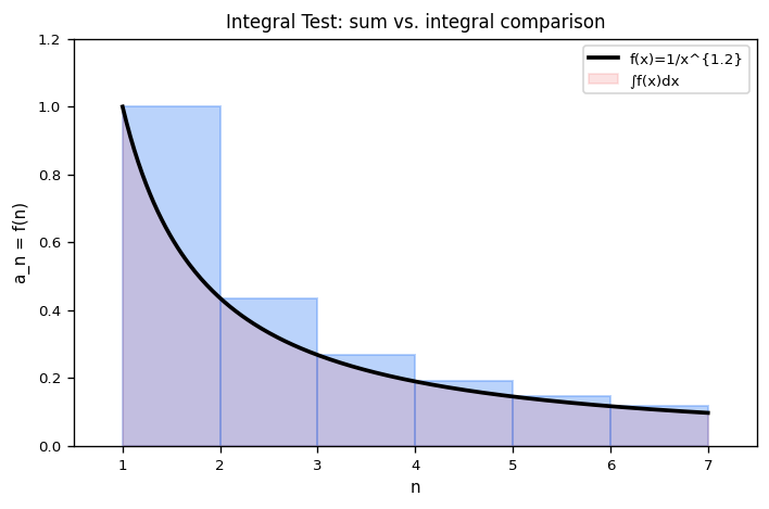
5.6 Integral Test
Theorem 8 (Integral Test). Let \(f\) be continuous, positive, and decreasing on \([1,\infty)\), with \(a_n = f(n)\). Then:
(i) \(\int_1^{n+1} f(x)\,dx \le S_n \le a_1 + \int_1^n f(x)\,dx\).
(ii) \(\sum_{k=1}^\infty a_k\) converges if and only if \(\int_1^\infty f(x)\,dx\) converges.
(iii) If the series converges to \(S\), then \(\int_{n+1}^\infty f(x)\,dx \le S - S_n \le \int_n^\infty f(x)\,dx\).
Theorem 9 (\(p\)-Series Test). The series \(\sum_{n=1}^\infty \frac{1}{n^p}\) converges if and only if \(p > 1\).
5.7 Alternating Series
Definition (Alternating Series). A series of the form \(\sum_{n=1}^\infty (-1)^{n-1}a_n\) (or \(\sum (-1)^n a_n\)) with \(a_n > 0\) is called alternating.
Theorem 10 (Alternating Series Test). If (1) \(a_n > 0\), (2) \(a_{n+1} \le a_n\), and (3) \(\lim_{n\to\infty} a_n = 0\), then \(\sum_{n=1}^\infty (-1)^{n-1}a_n\) converges. Moreover, \(|S_k - S| \le a_{k+1}\).
5.8 Absolute vs. Conditional Convergence
Definition (Absolute and Conditional Convergence). A series \(\sum a_n\) converges absolutely if \(\sum |a_n|\) converges. It converges conditionally if \(\sum a_n\) converges but \(\sum |a_n|\) diverges.
Theorem 11 (Absolute Convergence Theorem). If \(\sum |a_n|\) converges, then \(\sum a_n\) converges.
Definition (Rearrangement). Given \(\sum a_n\) and a bijection \(\varphi:\mathbb{N}\to\mathbb{N}\), the series \(\sum b_n\) with \(b_n = a_{\varphi(n)}\) is a rearrangement of \(\sum a_n\).
Theorem 12 (Rearrangement Theorem).
If \(\sum a_n\) converges absolutely and \(\sum b_n\) is any rearrangement, then \(\sum b_n\) converges and \(\sum b_n = \sum a_n\).
If \(\sum a_n\) converges conditionally, then for any \(\alpha \in \mathbb{R}\) (or \(\alpha = \pm\infty\)), there exists a rearrangement \(\sum b_n\) with \(\sum b_n = \alpha\).
5.9 Ratio Test
Theorem 13 (Ratio Test). Given \(\sum a_n\), suppose \(\lim_{n\to\infty}\left|\frac{a_{n+1}}{a_n}\right| = L\).
If \(0 \le L < 1\), the series converges absolutely.
If \(L > 1\), the series diverges.
If \(L = 1\), no conclusion is possible.
The Ratio Test is particularly effective for series involving factorials or exponentials. It fails for ratios of polynomials.
Theorem 14 (Polynomial vs. Factorial Growth). For any \(x \in \mathbb{R}\), \(\lim_{n\to\infty}\frac{x^n}{n!} = 0\).
The order of magnitude hierarchy is: \(\ln(n) \ll n^p \ll x^n \ll n! \ll n^n\) for \(|x|>1\).
Chapter 6: Power Series
6.1 Introduction to Power Series
Definition (Power Series). A power series centered at \(x = a\) is \(\sum_{n=0}^\infty a_n(x-a)^n\), where \(x\) is a variable and \(a_n\) is the coefficient of \((x-a)^n\).
Definition (Interval and Radius of Convergence). The interval of convergence \(I\) is the set of \(x_0\) where \(\sum |a_n(x_0-a)^n|\) converges. The radius of convergence is \(R = \text{lub}(\{|x_0-a| : x_0 \in I\})\) (or \(R = \infty\) if \(I\) is unbounded).
Theorem 1 (Fundamental Convergence Theorem for Power Series). Given \(\sum a_n(x-a)^n\) with radius \(R\):
If \(R = 0\), the series converges only at \(x = a\).
If \(0 < R < \infty\), the series converges absolutely for \(|x-a| < R\) and diverges for \(|x-a| > R\).
If \(R = \infty\), the series converges absolutely for all \(x \in \mathbb{R}\).
The interval of convergence may or may not include the endpoints.
6.1.1 Finding the Radius of Convergence
Theorem 2 (Test for Radius of Convergence). If \(\lim_{n\to\infty}\left|\frac{a_{n+1}}{a_n}\right| = L\), then:
If \(0 < L < \infty\), then \(R = \frac{1}{L}\).
If \(L = 0\), then \(R = \infty\).
If \(L = \infty\), then \(R = 0\).
Theorem 3 (Equivalence of Radius of Convergence). If \(p\) and \(q\) are non-zero polynomials with \(q(n) \ne 0\) for \(n \ge k\), then \(\sum a_n(x-a)^n\) and \(\sum a_n\frac{p(n)}{q(n)}(x-a)^n\) have the same radius of convergence (though possibly different intervals).
6.2 Functions Represented by Power Series
Definition (Functions Represented by Power Series). If \(\sum a_n(x-a)^n\) has interval of convergence \(I\), then \(f(x) = \sum_{n=0}^\infty a_n(x-a)^n\) defines a function on \(I\).
Theorem 4 (Abel’s Theorem: Continuity of Power Series). If \(f(x) = \sum a_n(x-a)^n\) on the interval of convergence \(I\), then \(f\) is continuous on \(I\).
6.3 Differentiation of Power Series
Definition (Formal Derivative). The formal derivative of \(\sum_{n=0}^\infty a_n(x-a)^n\) is \(\sum_{n=1}^\infty n\,a_n(x-a)^{n-1}\).
Theorem 5 (Term-by-Term Differentiation). If \(\sum a_n(x-a)^n\) has radius \(R > 0\) and \(f(x) = \sum_{n=0}^\infty a_n(x-a)^n\) for \(|x-a| < R\), then \(f\) is differentiable on \((a-R, a+R)\) and
\[ f'(x) = \sum_{n=1}^\infty n\,a_n(x-a)^{n-1}. \]Repeated application shows \(f\) has derivatives of all orders on \((a-R, a+R)\), with \(f^{(k)}(x) = \sum_{n=k}^\infty n(n-1)\cdots(n-k+1)\,a_n(x-a)^{n-k}\).
As an important application, since \(g(x) = \sum_{n=0}^\infty \frac{x^n}{n!}\) satisfies \(g'(x) = g(x)\), we deduce \(e^x = \sum_{n=0}^\infty \frac{x^n}{n!}\) for all \(x \in \mathbb{R}\).
6.4 Integration of Power Series
Theorem 6 (Term-by-Term Integration). If \(f(x) = \sum_{n=0}^\infty a_n(x-a)^n\) with radius \(R > 0\), then for \(|x-a| < R\),
\[ \int f(x)\,dx = C + \sum_{n=0}^\infty a_n\frac{(x-a)^{n+1}}{n+1}. \]Definition (Uniqueness of Power Series Representations). If \(f(x) = \sum a_n(x-a)^n\) on an interval, then the coefficients are uniquely determined by \(a_n = \frac{f^{(n)}(a)}{n!}\).
6.5 Review of Taylor Polynomials
Definition (Taylor Polynomial). Assume \(f\) is \(n\)-times differentiable at \(x = a\). The \(n\)-th degree Taylor polynomial centered at \(a\) is
\[ T_{n,a}(x) = \sum_{k=0}^n \frac{f^{(k)}(a)}{k!}(x-a)^k. \]Theorem 7 (Taylor Polynomial Properties). The Taylor polynomial \(T_{n,a}(x)\) is the unique polynomial of degree \(\le n\) such that \(T_{n,a}^{(k)}(a) = f^{(k)}(a)\) for \(k = 0, 1, \ldots, n\).
6.6 Taylor’s Theorem and Error Estimates
Definition (Taylor Remainder). \(R_{n,a}(x) = f(x) - T_{n,a}(x)\).
Theorem 8 (Taylor’s Theorem). If \(f\) is \((n+1)\)-times differentiable on an interval \(I\) containing \(a\), then for each \(x \in I\) there exists \(c\) between \(x\) and \(a\) such that
\[ R_{n,a}(x) = \frac{f^{(n+1)}(c)}{(n+1)!}(x-a)^{n+1}. \]When \(n=0\), this reduces to the Mean Value Theorem. Taylor’s Theorem is the key tool for bounding approximation errors.
Theorem 9 (Taylor’s Approximation Theorem). If \(f^{(k+1)}\) is continuous on \([-1,1]\), there exists \(M > 0\) such that
\[ |f(x) - T_{k,0}(x)| \le M|x|^{k+1} \]for all \(x \in [-1,1]\).
6.7 Taylor Series
Definition (Taylor Series). If \(f\) has derivatives of all orders at \(a\), the Taylor series for \(f\) centered at \(a\) is \(\sum_{n=0}^\infty \frac{f^{(n)}(a)}{n!}(x-a)^n\). We write \(f(x) \sim \sum_{n=0}^\infty \frac{f^{(n)}(a)}{n!}(x-a)^n\). When \(a=0\), this is the Maclaurin series.
6.8 Convergence of Taylor Series
Theorem 10 (Convergence Theorem for Taylor Series). If \(f\) has derivatives of all orders on \(I\) containing \(a\), and there exists \(M\) with \(|f^{(k)}(x)| \le M\) for all \(k\) and \(x \in I\), then
\[ f(x) = \sum_{n=0}^\infty \frac{f^{(n)}(a)}{n!}(x-a)^n \]for all \(x \in I\).
Key Taylor series (valid for all \(x \in \mathbb{R}\)):
\[ e^x = \sum_{n=0}^\infty \frac{x^n}{n!}, \quad \cos(x) = \sum_{k=0}^\infty (-1)^k\frac{x^{2k}}{(2k)!}, \quad \sin(x) = \sum_{k=0}^\infty (-1)^k\frac{x^{2k+1}}{(2k+1)!}. \]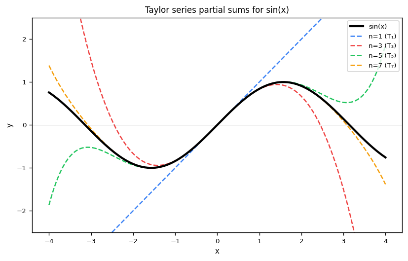
6.9 Binomial Series
Theorem 11 (Binomial Theorem). For \(a \in \mathbb{R}\) and \(n \in \mathbb{N}\),
\[ (a+x)^n = \sum_{k=0}^n \binom{n}{k}a^{n-k}x^k. \]Definition (Generalized Binomial Coefficients and Series). For \(\alpha \in \mathbb{R}\) and \(k \in \{0,1,2,\ldots\}\),
\[ \binom{\alpha}{k} = \frac{\alpha(\alpha-1)(\alpha-2)\cdots(\alpha-k+1)}{k!} \]with \(\binom{\alpha}{0} = 1\). The generalized binomial series is \(\sum_{k=0}^\infty \binom{\alpha}{k}x^k\).
Theorem 12 (Generalized Binomial Theorem). For \(\alpha \in \mathbb{R}\) and \(|x| < 1\),
\[ (1+x)^\alpha = \sum_{k=0}^\infty \binom{\alpha}{k}x^k. \]6.10 Additional Applications
Important derived series (for \(|x| \le 1\)):
\[ \arctan(x) = \sum_{n=0}^\infty (-1)^n\frac{x^{2n+1}}{2n+1} \]which yields Leibniz’s formula \(\pi = 4\left(1 - \frac{1}{3} + \frac{1}{5} - \frac{1}{7} + \cdots\right)\).
Chapter 7: Curves
7.1 Vector-Valued Functions
A vector-valued function \(\vec{F}(t): I \subseteq \mathbb{R} \to \mathbb{R}^2\) is written \(\vec{F}(t) = (x(t), y(t))\), where \(x(t)\) and \(y(t)\) are the coordinate functions. The range of \(\vec{F}\) is called a curve; arrows indicate orientation.
7.2 Limits and Continuity
Definition (Limit of a Vector-Valued Function). We say \(\lim_{t\to t_0}\vec{F}(t) = \vec{L} = (L_1, L_2)\) if for every \(\varepsilon > 0\) there exists \(\delta > 0\) such that \(0 < |t-t_0| < \delta\) implies the distance from \(\vec{F}(t)\) to \(\vec{L}\) is less than \(\varepsilon\).
Theorem 1 (Limit Theorem). \(\lim_{t\to t_0}\vec{F}(t) = (L_1, L_2)\) if and only if \(\lim_{t\to t_0}x(t) = L_1\) and \(\lim_{t\to t_0}y(t) = L_2\).
Definition (Continuity). \(\vec{F}(t)\) is continuous at \(t_0\) if \(\lim_{t\to t_0}\vec{F}(t)\) exists and equals \(\vec{F}(t_0)\).
Theorem 2 (Continuity Theorem). \(\vec{F}(t) = (x(t), y(t))\) is continuous at \(t_0\) if and only if both \(x(t)\) and \(y(t)\) are continuous at \(t_0\).
7.3 Derivatives and Velocity
Definition (Instantaneous Velocity). If \(\vec{F}(t)\) is the position at time \(t\), the instantaneous velocity is
\[ \vec{v} = \lim_{\Delta t \to 0}\frac{\vec{F}(t_0+\Delta t) - \vec{F}(t_0)}{\Delta t}. \]7.4 Derivatives and Tangent Lines
Definition (Derivative of a Vector-Valued Function).
\[ \vec{F}'(t_0) = \lim_{\Delta t \to 0}\frac{\vec{F}(t_0+\Delta t) - \vec{F}(t_0)}{\Delta t}. \]Definition (Tangent Line). If \(\vec{F}'(t_0) \ne (0,0)\), the tangent line to \(\vec{F}\) at \(t_0\) is
\[ \vec{w} = \vec{F}(t_0) + \alpha\,\vec{F}'(t_0). \]Theorem 3 (Differentiation Theorem). \(\vec{F}(t) = (x(t), y(t))\) is differentiable at \(t_0\) if and only if both \(x(t)\) and \(y(t)\) are differentiable at \(t_0\), and \(\vec{F}'(t_0) = (x'(t_0), y'(t_0))\).
A curve is smooth at \(t_0\) if \(\vec{F}'(t_0)\) exists and \(\vec{F}'(t_0) \ne (0,0)\).
7.5 Linear Approximation
Definition (Linear Approximation). If \(\vec{F}(t)\) is differentiable at \(t_0\) with \(\vec{F}'(t_0) \ne (0,0)\), the linear approximation is
\[ \vec{L}_{t_0}(t) = \vec{F}(t_0) + (t - t_0)\,\vec{F}'(t_0). \]This satisfies \(\vec{L}_{t_0}(t_0) = \vec{F}(t_0)\) and \(\vec{L}'_{t_0}(t_0) = \vec{F}'(t_0)\), and its range is the tangent line.
7.6 Arc Length of a Curve
For a continuously differentiable \(\vec{F}(t) = (x(t), y(t))\), the arc length over \([a,b]\) is
\[ S = \int_a^b \|\vec{F}'(t)\|\,dt = \int_a^b \sqrt{(x'(t))^2 + (y'(t))^2}\,dt. \]Since \(\|\vec{F}'(t)\|\) is the speed, this says distance = \(\int\)(speed)\(\,dt\). For curves of the form \(\vec{F}(t) = (t, f(t))\), this reduces to the arc length formula \(\int_a^b \sqrt{1+(f'(t))^2}\,dt\).
