These notes cover MATH 147 (Calculus 1 for Honours Mathematics) at the University of Waterloo. The course is the rigorous companion to MATH 137: every definition is given the full \(\varepsilon\)-\(\delta\) treatment, every major theorem is proved, and the real number system itself is developed from first principles. The primary inspiration is Spivak’s Calculus and Rudin’s Principles of Mathematical Analysis, but the presentation is aimed at a student encountering rigorous analysis for the first time.

---

Chapter 1: The Real Number System

The calculus we develop in this course — limits, derivatives, integrals — ultimately rests on properties of the real numbers \(\mathbb{R}\). Most of us use real numbers every day without asking what they actually are. In MATH 147, we take that question seriously. The key insight is that \(\mathbb{R}\) is not just an algebraic object (a field) or an ordered object (like \(\mathbb{Q}\)), but a complete ordered field, and it is completeness that makes calculus possible.

1.1 Ordered Fields

An ordered field is a set equipped with addition, multiplication, and an ordering that all interact in the expected ways. The rationals \(\mathbb{Q}\) form an ordered field, but as we will see, they are fundamentally insufficient for analysis.

Both \(\mathbb{Q}\) and \(\mathbb{R}\) are ordered fields. The key difference comes next.

1.2 The Least Upper Bound Property

The rational numbers have a glaring gap: the set \(\{x \in \mathbb{Q} : x^2 < 2\}\) is bounded above in \(\mathbb{Q}\) (by \(2\), say), yet has no least upper bound in \(\mathbb{Q}\). The real numbers are distinguished precisely by the fact that this cannot happen.

We take this as an axiom characterising \(\mathbb{R}\): up to isomorphism of ordered fields, there is exactly one complete ordered field, and we call it the real numbers. Notice that the completeness axiom fails for \(\mathbb{Q}\): the set \(\{q \in \mathbb{Q} : q > 0, q^2 < 2\}\) has no supremum in \(\mathbb{Q}\).

1.3 Consequences: Archimedean Property and Density of \(\mathbb{Q}\)

Completeness has far-reaching consequences. Two of the most important are that \(\mathbb{N}\) is not bounded in \(\mathbb{R}\), and that between any two real numbers lies a rational.

Proof. If \(\mathbb{N}\) were bounded above in \(\mathbb{R}\), then by completeness \(\alpha = \sup \mathbb{N}\) would exist. Since \(\alpha - 1\) is not an upper bound, there is some \(n \in \mathbb{N}\) with \(n > \alpha - 1\), giving \(n + 1 > \alpha\). But \(n+1 \in \mathbb{N}\), contradicting that \(\alpha\) is an upper bound. \(\square\)

Proof. By the Archimedean property, choose \(n \in \mathbb{N}\) with \(n > 1/(b-a)\), so \(1/n < b - a\). Let \(m = \lfloor na \rfloor + 1\), so \(m - 1 \le na < m\), giving \(a < m/n \le a + 1/n < a + (b-a) = b\). Then \(q = m/n\) works. \(\square\)

The triangle inequality is the single most-used estimate in all of analysis. Every \(\varepsilon\)-\(\delta\) proof eventually invokes it.

---

Chapter 2: Sequences

A sequence is the simplest setting in which to develop the idea of a limit. Before we can meaningfully speak of a function approaching a value, we need a rigorous account of what it means for a list of numbers to converge. The theory of sequences also provides the tools to prove completeness consequences like the Bolzano–Weierstrass theorem, which will be indispensable later.

2.1 Limits of Sequences

The key idea is that \(\varepsilon\) is given first — it is the tolerance — and we must respond with an \(N\) that works for that tolerance. The order matters: \(N\) is allowed to depend on \(\varepsilon\).

Proof. Suppose \(L \ne M\); set \(\varepsilon = |L - M|/2 > 0\). Choose \(N_1\) so that \(n \ge N_1\) implies \(|a_n - L| < \varepsilon\), and \(N_2\) so that \(n \ge N_2\) implies \(|a_n - M| < \varepsilon\). For \(n \ge \max(N_1, N_2)\), the triangle inequality gives \(|L - M| \le |L - a_n| + |a_n - M| < 2\varepsilon = |L - M|\), a contradiction. \(\square\)

2.2 Limit Theorems

2.3 Monotone Convergence Theorem

This is where completeness first pays off for sequences. A monotone sequence that is bounded has nowhere to go but converge.

Proof. Let \(L = \sup\{a_n\}\), which exists by completeness. Given \(\varepsilon > 0\), since \(L - \varepsilon\) is not an upper bound, there exists \(a_N > L - \varepsilon\). Since the sequence is increasing, for all \(n \ge N\) we have \(L - \varepsilon < a_N \le a_n \le L\), so \(|a_n - L| < \varepsilon\). \(\square\)

The Monotone Convergence Theorem is the engine behind many existence arguments: to prove a sequence converges, it often suffices to show it is monotone and bounded.

2.4 Subsequences and the Bolzano–Weierstrass Theorem

The contrapositive is equally important: if two subsequences converge to different limits, the original sequence diverges.

Proof. Let \(\{a_n\} \subset [A, B]\). We perform repeated bisection. Set \([A_0, B_0] = [A, B]\). Given \([A_k, B_k]\), at least one of \([A_k, \tfrac{A_k+B_k}{2}]\) or \([\tfrac{A_k+B_k}{2}, B_k]\) contains infinitely many terms; call it \([A_{k+1}, B_{k+1}]\). Pick \(n_{k+1} > n_k\) with \(a_{n_{k+1}} \in [A_{k+1}, B_{k+1}]\). The nested intervals have length \((B-A)/2^k \to 0\), so by completeness they share a unique point \(L\). Since \(a_{n_k} \in [A_k, B_k]\) and the interval widths shrink to zero, \(a_{n_k} \to L\). \(\square\)

2.5 Cauchy Sequences

The Bolzano–Weierstrass theorem tells us bounded sequences have convergent subsequences, but how can we verify convergence without knowing the limit in advance? Cauchy sequences answer this.

The definition says the terms of the sequence eventually cluster together, without reference to any putative limit.

Proof. (\(\Rightarrow\)) If \(a_n \to L\), given \(\varepsilon > 0\) choose \(N\) so that \(|a_n - L| < \varepsilon/2\) for \(n \ge N\). Then \(|a_m - a_n| \le |a_m - L| + |L - a_n| < \varepsilon\).

(\(\Leftarrow\)) Let \(\{a_n\}\) be Cauchy. First, every Cauchy sequence is bounded (choose \(N\) for \(\varepsilon = 1\); then \(|a_n| \le |a_N| + 1\) for \(n \ge N\), and the finitely many earlier terms are also bounded). By Bolzano–Weierstrass, there is a convergent subsequence \(a_{n_k} \to L\). Given \(\varepsilon > 0\), choose \(N\) so that \(m, n \ge N\) implies \(|a_m - a_n| < \varepsilon/2\), and \(K\) so that \(k \ge K\) implies \(|a_{n_k} - L| < \varepsilon/2\). For \(n \ge N\), pick \(k \ge K\) with \(n_k \ge N\); then \(|a_n - L| \le |a_n - a_{n_k}| + |a_{n_k} - L| < \varepsilon\). \(\square\)

This equivalence — Cauchy iff convergent — is another way of stating completeness. In the rationals, Cauchy sequences need not converge (e.g.\ the rational approximations to \(\sqrt{2}\)).

---

Chapter 3: Limits and Continuity

With sequences in hand, we can define limits of functions. The interplay between function limits and sequential limits is both elegant and practically powerful: many properties of function limits reduce immediately to the corresponding sequence results.

3.1 The Epsilon-Delta Definition

Notice the condition \(0 < |x - a|\): we never evaluate \(f\) at \(x = a\). The limit is about the behaviour of \(f\) near \(a\), not at \(a\).

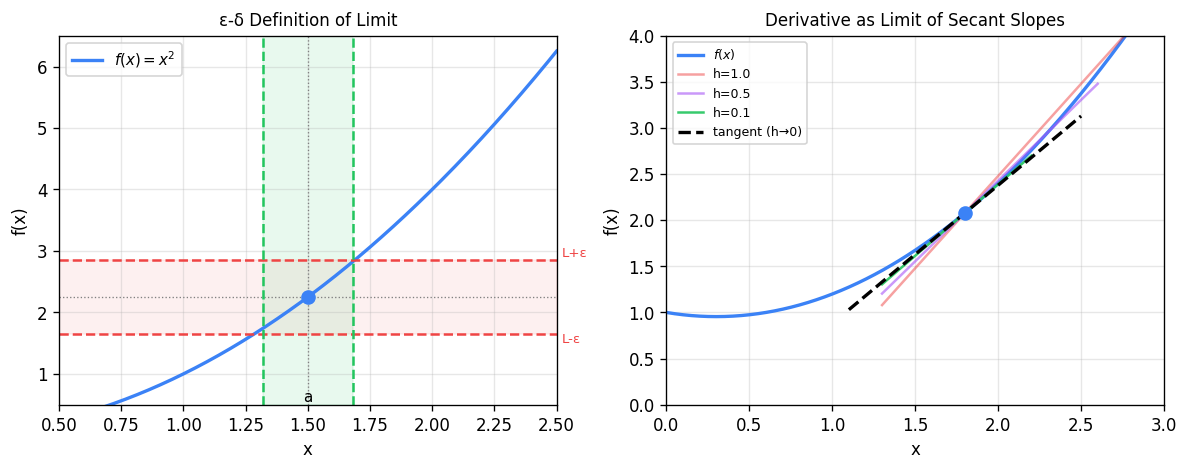
Left: the ε-δ definition of limit. The green vertical strip of width \(2\delta\) centred at \(a\) maps into the red horizontal band of height \(2\varepsilon\) around \(L\). Right: the derivative as the limiting slope of secant lines as \(h \to 0\); successive secant slopes (red, purple, green) converge to the tangent (black dashed).

3.2 Limit Laws

This theorem is the bridge between sequence theory and function limits. It means every result we proved for sequences carries over to function limits immediately.

Proof (sketch). For \(0 < \theta < \pi/2\), comparing areas of triangles and the circular sector on the unit circle gives \(\sin\theta < \theta < \tan\theta\), hence \(\cos\theta < \sin\theta/\theta < 1\). Since \(\cos\theta \to 1\), the Squeeze Theorem finishes it. \(\square\)

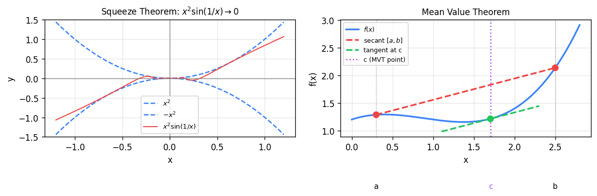
Left: the squeeze theorem in action — \(x^2\sin(1/x)\) (red) is sandwiched between \(-x^2\) and \(x^2\) (blue dashed), forcing the limit to 0 at the origin. Right: the MVT guarantees a point \(c\) (purple) where the tangent (green) is parallel to the secant through \((a, f(a))\) and \((b, f(b))\) (red dashed).

3.3 One-Sided Limits and Limits at Infinity

3.4 Continuity

The elementary functions — polynomials, \(\sin x\), \(\cos x\), \(e^x\), \(\ln x\) — are all continuous on their natural domains. Combining them with the theorem above produces a vast class of continuous functions.

3.5 The Intermediate Value Theorem

The IVT captures the geometric intuition that a continuous function cannot jump: if \(f\) is \(2\) at one point and \(7\) at another, it must take every value in between. This seemingly obvious fact requires completeness to prove.

Proof. Without loss of generality assume \(f(a) < k < f(b)\). Define \(S = \{x \in [a,b] : f(x) \le k\}\). Then \(a \in S\) so \(S \ne \emptyset\), and \(S\) is bounded above by \(b\). By completeness, \(c = \sup S\) exists. We claim \(f(c) = k\).

Suppose \(f(c) < k\). Since \(f\) is continuous at \(c\), with \(\varepsilon = k - f(c) > 0\) we find \(\delta > 0\) such that \(|x - c| < \delta\) implies \(|f(x) - f(c)| < \varepsilon\), i.e.\ \(f(x) < k\). Thus \([c, c+\delta) \subset S\) (as long as \(c + \delta \le b\)), contradicting that \(c\) is an upper bound for \(S\). Suppose \(f(c) > k\). Then by continuity, \(f(x) > k\) near \(c\), so \(c - \delta\) is also an upper bound of \(S\), contradicting \(c = \sup S\). Therefore \(f(c) = k\). \(\square\)

The IVT has powerful applications: it guarantees roots of polynomials of odd degree, underpins the bisection method for root-finding, and shows that continuous images of intervals are intervals.

3.6 The Extreme Value Theorem

The IVT tells us about intermediate values; the Extreme Value Theorem tells us about maximum and minimum values. Both require the interval to be closed and bounded, and both fail without these hypotheses.

Proof. Let \(M = \sup\{f(x) : x \in [a,b]\}\), which is finite by the claim below. Choose \(x_n \in [a,b]\) with \(f(x_n) > M - 1/n\). By Bolzano–Weierstrass, \(\{x_n\}\) has a convergent subsequence \(x_{n_k} \to x_{\max} \in [a,b]\) (the limit is in \([a,b]\) since the interval is closed). By continuity, \(f(x_{n_k}) \to f(x_{\max})\); since \(f(x_{n_k}) \to M\), we get \(f(x_{\max}) = M\). The minimum is handled similarly. That \(M < \infty\): if not, pick \(x_n\) with \(f(x_n) > n\); extract a convergent subsequence to \(x^*\); continuity forces \(f(x_n) \to f(x^*)\), contradicting \(f(x_n) \to \infty\). \(\square\)

3.7 Uniform Continuity

Ordinary continuity allows \(\delta\) to depend on both \(\varepsilon\) and the point \(a\). Uniform continuity is a stronger condition requiring a single \(\delta\) that works everywhere at once.

Proof. Suppose for contradiction that \(f\) is not uniformly continuous on \([a,b]\). Then there exists \(\varepsilon_0 > 0\) and sequences \(x_n, y_n \in [a,b]\) with \(|x_n - y_n| < 1/n\) but \(|f(x_n) - f(y_n)| \ge \varepsilon_0\). By Bolzano–Weierstrass, extract a convergent subsequence \(x_{n_k} \to c \in [a,b]\). Then \(y_{n_k} \to c\) too (since \(|x_{n_k} - y_{n_k}| \to 0\)). By continuity of \(f\) at \(c\), \(f(x_{n_k}) \to f(c)\) and \(f(y_{n_k}) \to f(c)\), so \(|f(x_{n_k}) - f(y_{n_k})| \to 0\), contradicting \(\ge \varepsilon_0\). \(\square\)

---

Chapter 4: Differentiation

Differentiation is the mathematical formalization of the notion of instantaneous rate of change. The derivative at a point is a limit — a single real number — that encodes the slope of the tangent line, the velocity of a moving particle, the sensitivity of an output to a change in input. What makes differentiation powerful is that it is local: the derivative at \(a\) depends only on the behaviour of \(f\) near \(a\).

4.1 The Derivative

Geometrically, \(f'(a)\) is the slope of the tangent line to the graph of \(f\) at the point \((a, f(a))\). The tangent line itself is \(y = f(a) + f'(a)(x - a)\), the best linear approximation to \(f\) near \(a\).

Proof. Write \(f(x) - f(a) = \frac{f(x)-f(a)}{x-a} \cdot (x-a)\). As \(x \to a\), the first factor tends to \(f'(a)\) and the second to \(0\), so the product tends to \(0\). \(\square\)

The converse is false: \(f(x) = |x|\) is continuous everywhere but not differentiable at \(0\), since \((|h| - 0)/h = \pm 1\) depending on the sign of \(h\).

4.2 Differentiation Rules

\[ \frac{d}{dx}\sin x = \cos x, \quad \frac{d}{dx}\cos x = -\sin x, \quad \frac{d}{dx} e^x = e^x, \quad \frac{d}{dx}\ln x = \frac{1}{x}. \]

4.3 The Chain Rule

The chain rule is perhaps the most important differentiation rule, governing how derivatives compose. Its proof requires care because the naive approach (dividing by \(g(x) - g(a)\)) fails when \(g(x) = g(a)\) at a sequence of points converging to \(a\).

\[ \phi(y) = \begin{cases} \dfrac{g(y) - g(f(a))}{y - f(a)} & y \ne f(a) \\ g'(f(a)) & y = f(a). \end{cases} \]\[ h(x) - h(a) = g(f(x)) - g(f(a)) = \phi(f(x)) \cdot (f(x) - f(a)). \]

Dividing by \(x - a\) (for \(x \ne a\)) and taking \(x \to a\): \(f(x) \to f(a)\) (by continuity), so \(\phi(f(x)) \to \phi(f(a)) = g'(f(a))\), and \((f(x)-f(a))/(x-a) \to f'(a)\). \(\square\)

4.4 Implicit Differentiation and Inverse Functions

When a relation \(F(x,y) = 0\) defines \(y\) implicitly as a differentiable function of \(x\), we differentiate both sides with respect to \(x\) using the Chain Rule on \(y\)-terms, then solve for \(dy/dx\). This technique gives us derivatives of inverse functions.

Applying this to \(f(x) = e^x\) (so \(g = \ln\)) gives \((\ln x)' = 1/x\). Applying to \(f(x) = \sin x\) on \([-\pi/2, \pi/2]\) gives \((\arcsin x)' = 1/\sqrt{1-x^2}\); similarly \((\arctan x)' = 1/(1+x^2)\).

4.5 Higher Derivatives

The second derivative measures concavity: \(f'' > 0\) on \(I\) means the graph bends upward (concave up), while \(f'' < 0\) means it bends downward. An inflection point is where concavity changes.

---

Chapter 5: The Mean Value Theorem and Applications

The Mean Value Theorem is the central result of one-variable differential calculus. It connects the local notion of a derivative at a point to the global behaviour of a function over an interval. Most of the key applications of differentiation — monotonicity, L’Hôpital’s Rule, Taylor’s theorem — ultimately flow from it.

5.1 Rolle’s Theorem and the MVT

Proof. By the EVT, \(f\) attains a maximum and minimum on \([a,b]\). If both are attained at the endpoints, then \(f\) is constant (since \(f(a)=f(b)\)) and \(f' \equiv 0\) on \((a,b)\). Otherwise, at least one extreme value is attained at an interior point \(c \in (a,b)\); at such a point the Local Extrema Theorem forces \(f'(c) = 0\). \(\square\)

Proof. Apply Rolle’s Theorem to the auxiliary function \(g(x) = f(x) - \frac{f(b)-f(a)}{b-a}(x-a)\). One checks \(g(a) = g(b) = f(a)\), so there is \(c\) with \(g'(c) = 0\), giving the result. \(\square\)

Geometrically, the MVT says the tangent line at some interior point is parallel to the secant through the endpoints. Analytically, it says the instantaneous rate of change equals the average rate of change at some moment — a rigorous form of the intuition that a car traveling 60 km in one hour must at some instant be going exactly 60 km/h.

5.2 Monotonicity

Proof. For (i), let \(a \le x_1 < x_2 \le b\). By the MVT there is \(c \in (x_1, x_2)\) with \(f(x_2) - f(x_1) = f'(c)(x_2 - x_1) > 0\). \(\square\)

5.3 L’Hôpital’s Rule

L’Hôpital’s Rule handles indeterminate forms \(0/0\) and \(\infty/\infty\) by replacing the ratio of functions with the ratio of their derivatives. Its proof uses the Cauchy Mean Value Theorem.

Proof. Apply Rolle’s to \(h(x) = [f(b)-f(a)]g(x) - [g(b)-g(a)]f(x)\). Then \(h(a) = f(b)g(a) - f(a)g(b) = h(b)\), so there is \(c\) with \(h'(c) = 0\). \(\square\)

\[ \frac{f(x)}{g(x)} = \frac{f(x) - f(a)}{g(x) - g(a)} = \frac{f'(c_x)}{g'(c_x)}. \]

As \(x \to a^+\), we have \(c_x \to a^+\), and hence \(f'(c_x)/g'(c_x) \to L\). \(\square\)

The most frequently used instances: \(\lim_{x\to 0}\frac{\sin x}{x} = 1\), \(\lim_{x\to\infty}\frac{\ln x}{x} = 0\), \(\lim_{x\to\infty}\frac{x^n}{e^x} = 0\).

5.4 Convexity

---

Chapter 6: Taylor Polynomials and Approximation

The derivative captures the first-order behaviour of a function near a point. Higher derivatives capture higher-order behaviour, and Taylor’s theorem lets us assemble all of this information into a polynomial approximation with a quantitative error bound. This is the starting point for numerical analysis, asymptotic analysis, and eventually the theory of power series.

6.1 Taylor Polynomials

Notice that \(T_{n,a}\) is the unique polynomial of degree at most \(n\) whose first \(n\) derivatives at \(a\) match those of \(f\): \(T_{n,a}^{(k)}(a) = f^{(k)}(a)\) for \(k = 0, 1, \ldots, n\). The case \(n = 1\) recovers the linear (tangent line) approximation.

\[ e^x = \sum_{k=0}^{n} \frac{x^k}{k!} + R_n(x), \quad \sin x = \sum_{k=0}^{m} \frac{(-1)^k x^{2k+1}}{(2k+1)!} + R_{2m+1}(x), \]\[ \cos x = \sum_{k=0}^{m} \frac{(-1)^k x^{2k}}{(2k)!} + R_{2m}(x), \quad \frac{1}{1-x} = \sum_{k=0}^{n} x^k + R_n(x) \text{ for } |x| < 1. \]

6.2 Taylor’s Theorem with Remainder

\[ g(t) = f(x) - T_{n,t}(x) - M(x-t)^{n+1}. \]

One checks that \(g(x) = 0\) and \(g(a) = 0\) (by construction of \(M\)). Computing \(g'(t)\): the terms in \(T_{n,t}(x)\) telescope when differentiated with respect to \(t\), leaving \(g'(t) = -\frac{f^{(n+1)}(t)}{n!}(x-t)^n + M(n+1)(x-t)^n\). By Rolle’s Theorem applied to \(g\) on the interval with endpoints \(a\) and \(x\), there is \(c\) with \(g'(c) = 0\), giving \(M = f^{(n+1)}(c)/(n+1)!\). \(\square\)

When \(n = 0\), Taylor’s Theorem reduces to the Mean Value Theorem. The Lagrange form of the remainder is what makes Taylor polynomials useful: if we can bound \(|f^{(n+1)}|\), we get a concrete error bound.

6.3 Applications

---

Chapter 7: Series

An infinite series is a sum with infinitely many terms. This is not a priori a well-defined operation, and its meaning must be defined through limits of partial sums. The key questions are: when does a series converge, and how do its properties (like absolute vs.\ conditional convergence) affect that?

7.1 Convergence of Series

Proof. If \(S_k \to S\), then \(a_n = S_n - S_{n-1} \to S - S = 0\). \(\square\)

The converse is famously false: \(\sum 1/n\) diverges (the harmonic series) despite \(1/n \to 0\).

7.2 Geometric and \(p\)-Series

Proof. Partial sums satisfy \(S_k = (1 - r^{k+1})/(1-r)\) when \(r \ne 1\). If \(|r| < 1\), \(r^{k+1} \to 0\); if \(|r| \ge 1\), the terms do not tend to zero. \(\square\)

The divergence of \(\sum 1/n\) (\(p = 1\)) can be seen by grouping: \(1 + 1/2 + (1/3 + 1/4) + (1/5 + \cdots + 1/8) + \cdots\), where each group sums to at least \(1/2\).

7.3 Convergence Tests

Proof. The even partial sums \(S_{2k}\) are increasing and bounded above by \(S_1 = b_1\); the odd partial sums \(S_{2k+1}\) are decreasing and bounded below by \(S_2\). Both subsequences converge, and since \(S_{2k+1} - S_{2k} = b_{2k+1} \to 0\), they share the same limit \(S\). \(\square\)

7.4 Absolute and Conditional Convergence

The distinction between absolute and conditional convergence is one of the deeper surprises of series theory.

Proof. Define \(b_n = a_n + |a_n|\), so \(0 \le b_n \le 2|a_n|\). Since \(\sum |a_n|\) converges, so does \(\sum b_n\) by comparison. Then \(\sum a_n = \sum b_n - \sum |a_n|\) converges. \(\square\)

The archetypal conditionally convergent series is \(\sum_{n=1}^\infty (-1)^{n-1}/n = \ln 2\), which converges by the alternating series test but whose absolute values form the divergent harmonic series.

This theorem is genuinely shocking: by reordering the terms of a conditionally convergent series, we can make it sum to any value we like. The key is that for a conditionally convergent series, both the positive-term subseries and the negative-term subseries must diverge (to \(+\infty\) and \(-\infty\) respectively), providing unlimited “credit” and “debt” to spend.

By contrast, absolutely convergent series can be rearranged freely: every rearrangement converges to the same sum. This is why absolute convergence is the “safe” notion in analysis.

---

These notes cover the core material of MATH 147. The approach throughout has been to develop each concept rigorously while keeping the geometric and analytic intuition in the foreground. The completeness of \(\mathbb{R}\) is the invisible thread running through every major theorem: it gives us the Monotone Convergence Theorem, Bolzano–Weierstrass, the Cauchy Criterion, the Extreme Value Theorem, the Intermediate Value Theorem, and ultimately all the machinery of analysis.