CS 370: Numerical Computation
Jeff Orchard
Estimated study time: 56 minutes
Table of contents
Chapter 1: Floating Point Number Systems
Pitfalls in Floating Point Computation
Most mathematical courses assume that arithmetic is exact, operating over the real number line \(\mathbb{R}\). In practice, scientific computation runs on a computer’s floating point number system, a finite approximation to \(\mathbb{R}\) in which most real numbers can only be represented approximately. Two classic examples illustrate how this can go catastrophically wrong.
Example 1: A dangerous recurrence. Consider the integral
\[ I_n = \int_0^1 \frac{x^n}{x + \alpha} \, dx \]for constant parameter \(\alpha\). One can show that \(I_0 = \log\!\left(\frac{1+\alpha}{\alpha}\right)\) and the recurrence
\[ I_n = \frac{1}{n} - \alpha I_{n-1} \]holds. This seems like an efficient way to evaluate \(I_n\) for large \(n\): compute \(I_0\) and iterate. For \(\alpha = 0.5\) the computation gives a reasonable answer \(I_{100} \approx 6.64 \times 10^{-3}\), but for \(\alpha = 2.0\) it yields \(I_{100} \approx 2.1 \times 10^{22}\) — clearly wrong, since when \(x \in [0,1]\) and \(\alpha > 1\) the integrand satisfies \(\frac{x^n}{x+\alpha} \leq x^n\), so \(I_n \leq \frac{1}{n+1}\). The recurrence is perfectly correct mathematically, but is numerically unstable when \(|\alpha| > 1\).
Example 2: Catastrophic cancellation. To compute \(e^{-5.5}\) via its Taylor series, method 1 computes \(1 - 5.5 + 15.125 - 27.730 + \cdots\) directly, while method 2 evaluates \(\frac{1}{1 + 5.5 + 15.125 + \cdots}\). With five significant digits, method 1 yields \(0.0026363\) while method 2 yields \(0.0040865\) — the true answer is \(0.0040868\). Method 1 suffers from severe cancellation error: large positive and negative terms cancel, wiping out significant digits.
The Floating Point Number System
The real number system \(\mathbb{R}\) is infinite in two ways: unbounded in extent and infinitely dense. Computers can only represent finite sets of numbers. Every floating point number system is characterized by four integer parameters \(\{\beta, t, L, U\}\), where \(\beta\) is the base (typically 2 or 10), \(t\) is the number of significant digits in the mantissa, and \([L, U]\) is the exponent range. A nonzero floating point number has the normalized form
\[ \pm\, 0.d_1 d_2 \cdots d_t \times \beta^p, \quad L \leq p \leq U,\quad d_1 \neq 0. \]The two IEEE standards dominating modern hardware are:
| Standard | \(\beta\) | \(t\) | \(L\) | \(U\) |
|---|---|---|---|---|
| IEEE single precision | 2 | 24 | \(-126\) | 127 |
| IEEE double precision | 2 | 53 | \(-1022\) | 1023 |
Absolute and Relative Error
Given a computed result \(x\) and the correct value \(x_{\text{exact}}\), the absolute error is \(|x_{\text{exact}} - x|\) and the relative error is
\[ E_{\text{rel}} = \frac{|x_{\text{exact}} - x|}{|x_{\text{exact}}|}. \]The computed value \(x\) approximates \(x_{\text{exact}}\) to about \(s\) significant digits when \(0.5 \times 10^{-s} \leq E_{\text{rel}} < 5.0 \times 10^{-s}\). Relative error is the more useful measure for digital arithmetic because it quantifies correct significant digits independently of the magnitude of the numbers.
Machine Epsilon and the fl(x) Relation
An important consequence of floating point design is that the largest possible relative error in representing a real \(x\) by its floating point approximation \(fl(x)\) is bounded by a constant called machine epsilon (or unit round-off error):
\[ \varepsilon = \frac{1}{2}\,\beta^{1-t}. \]Equivalently, \(\varepsilon\) is the smallest representable number such that \(1 + \varepsilon > 1\). For any nonzero \(x\) in range,
\[ fl(x) = x(1 + \delta), \quad |\delta| \leq \varepsilon. \]This means every result of a single floating point operation \(\oplus\) satisfies
\[ w \oplus z = fl(w + z) = (w + z)(1 + \delta). \]IEEE arithmetic guarantees that each single operation produces the nearest representable floating point number to the exact real result. An exponent too large causes overflow; too negative causes underflow.
Cancellation and Round-off Error Analysis
Although individual floating point operations introduce relative errors at most \(\varepsilon\), cascading operations can amplify errors significantly. For a sum \(a + b + c\) computed as \((a \oplus b) \oplus c\), the relative error satisfies
\[ |E_{\text{rel}}| \leq \frac{|a| + |b| + |c|}{|a + b + c|}\,(2\varepsilon + \varepsilon^2). \]The condition number for this computation is \(\kappa = (|a|+|b|+|c|)/|a+b+c|\). When positive and negative terms nearly cancel — so that \(|a+b+c| \ll |a|+|b|+|c|\) — the condition number becomes huge and the relative error can be catastrophically large. This is cancellation error, the phenomenon that afflicted method 1 for \(e^{-5.5}\).
Conditioning and Stability
Conditioning is a property of the mathematical problem itself, independent of any algorithm. A problem is well-conditioned if a small relative change in the input produces only a proportionally small change in the output. It is ill-conditioned if small input perturbations can cause large output perturbations.
Stability is a property of an algorithm for solving a problem. An algorithm is stable if small errors introduced at any step (due to floating point arithmetic, data errors, or initial condition perturbations) remain bounded throughout the computation.
Stability analysis of the recurrence. In Example 1, let \(\tilde{I}_0 = I_0 + \epsilon_0\) (the true value plus a small initial error). Propagating through the recurrence \(I_n = \frac{1}{n} - \alpha I_{n-1}\) shows the error at step \(n\) satisfies \(\epsilon_n = (-\alpha)^n \epsilon_0\). When \(|\alpha| > 1\) the error grows exponentially — the algorithm is unstable. When \(|\alpha| < 1\) the error decays — the algorithm is stable. The fix for \(|\alpha| > 1\): run the recurrence backwards, starting from a reliable estimate for large \(n\) and working down to \(n = 0\), which is stable in that direction.
Chapter 2: Interpolation
Interpolation is the problem of constructing a function \(p(x)\) that exactly passes through a given set of data points \((x_1, y_1), \ldots, (x_n, y_n)\), so that \(p(x_i) = y_i\) for all \(i\). The interpolating function can then be used to estimate values at unknown points, compute derivatives, or serve as a component of larger numerical algorithms (integration, ODEs, optimization).
Polynomial Interpolation
Existence and uniqueness theorem: Given \(n\) data pairs \((x_i, y_i)\) with distinct \(x_i\), there is a unique polynomial \(p(x)\) of degree at most \(n-1\) that interpolates this data.
Vandermonde Systems
The most direct approach represents \(p(x) = c_1 + c_2 x + \cdots + c_n x^{n-1}\) and enforces \(p(x_i) = y_i\) for each \(i\). This produces the Vandermonde system \(V\mathbf{c} = \mathbf{y}\) where
\[ V = \begin{pmatrix} 1 & x_1 & \cdots & x_1^{n-1} \\ 1 & x_2 & \cdots & x_2^{n-1} \\ \vdots & & & \vdots \\ 1 & x_n & \cdots & x_n^{n-1} \end{pmatrix}. \]The matrix is nonsingular when the \(x_i\) are distinct (the determinant equals \(\prod_{i < j}(x_i - x_j) \neq 0\)), proving the uniqueness theorem.
Newton Divided Differences Form
The Newton form of the interpolating polynomial is built incrementally using divided differences. Given nodes \(x_0, x_1, \ldots, x_n\):
\[ p(x) = f[x_0] + f[x_0,x_1](x-x_0) + f[x_0,x_1,x_2](x-x_0)(x-x_1) + \cdots \]The divided differences are computed via the triangular table:
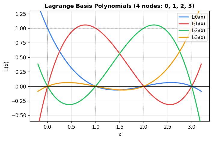
Lagrange Form
An elegant explicit construction uses Lagrange basis polynomials:
\[ L_k(x) = \prod_{\substack{j=1 \\ j \neq k}}^{n} \frac{x - x_j}{x_k - x_j}. \]Each \(L_k\) has the cardinal property \(L_k(x_j) = \delta_{kj}\). The interpolating polynomial is then
\[ p(x) = \sum_{k=1}^{n} y_k L_k(x). \]The Lagrange form is useful for theoretical analysis and for evaluation at a small number of points without solving a linear system.
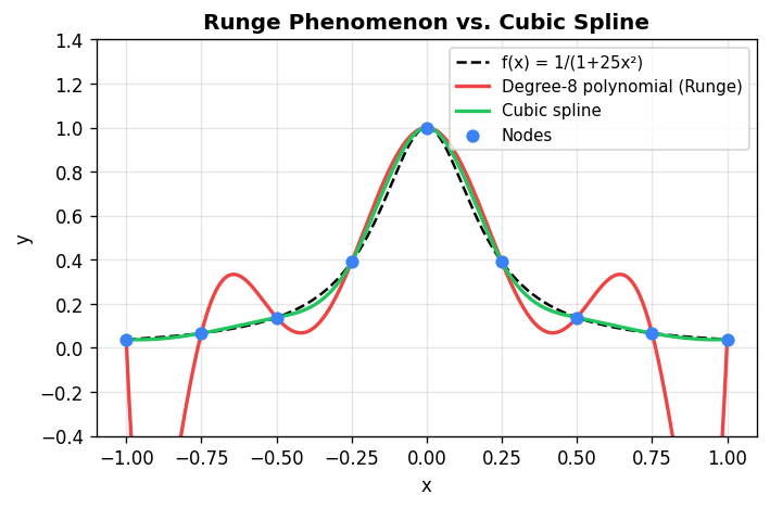
Piecewise Polynomial Interpolation
A single high-degree polynomial interpolant becomes problematic as the number of points grows: it tends to oscillate wildly between the data points (Runge’s phenomenon). The remedy is piecewise polynomial interpolation, where a different low-degree polynomial is used on each subinterval \([x_i, x_{i+1}]\). The result must be:
- an interpolant (\(p(x_i) = y_i\)),
- a polynomial on each subinterval,
- continuous across the full interval.
The simplest case is piecewise linear interpolation (linear \(p\) on each subinterval), which produces straight-line segments between consecutive data points. This is what MATLAB’s plot(x,y) draws. Its limitation: the derivative is discontinuous at the data points (sharp corners).
Piecewise Hermite Interpolation
Hermite interpolation specifies both function values and derivatives at the nodes. On each subinterval \([x_i, x_{i+1}]\), write a cubic polynomial in local form:
\[ p_i(x) = a_i + b_i(x - x_i) + c_i(x - x_i)^2 + d_i(x - x_i)^3. \]Requiring \(p_i(x_i) = y_i\), \(p_i(x_{i+1}) = y_{i+1}\), \(p_i'(x_i) = s_i\), \(p_i'(x_{i+1}) = s_{i+1}\) gives four equations for four unknowns, with solutions:
\[ a_i = y_i, \quad b_i = s_i, \quad c_i = \frac{3y_i' - 2s_i - s_{i+1}}{\Delta x_i}, \quad d_i = \frac{s_{i+1} + s_i - 2y_i'}{(\Delta x_i)^2}, \]where \(y_i' = (y_{i+1} - y_i)/\Delta x_i\) and \(\Delta x_i = x_{i+1} - x_i\). This guarantees continuity of \(p\) and \(p'\) at all knots, given prescribed derivative values \(s_i\).
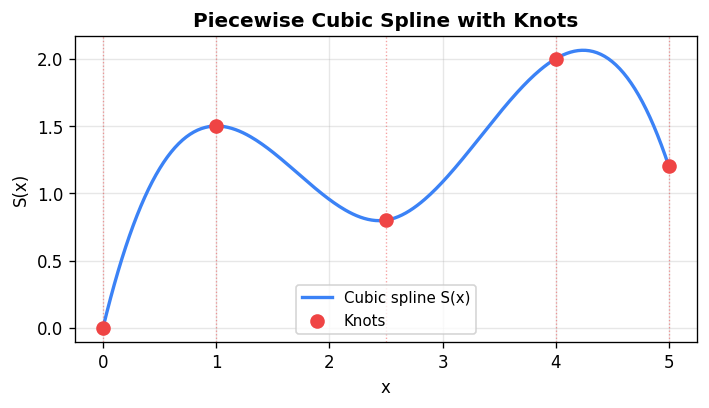
Spline Interpolants
A cubic spline \(S(x)\) is a piecewise cubic polynomial such that \(S(x)\), \(S'(x)\), and \(S''(x)\) are all continuous at the interior knots. This requires determining the unknown slopes \(s_i\) so that the second-derivative continuity condition \(S_i''(x_{i+1}) = S_{i+1}''(x_{i+1})\) is enforced. This yields a system of \(n-2\) equations:
\[ \Delta x_{i+1} s_{i-1} + 2(\Delta x_{i-1} + \Delta x_i) s_i + \Delta x_{i-1} s_{i+1} = 3(\Delta x_i y_{i-1}' + \Delta x_{i-1} y_i'), \quad i = 2, \ldots, n-1. \]Two boundary conditions must be added to close the system:
- Natural (free) boundary: \(S''(x_1) = 0\) and \(S''(x_n) = 0\) — models a “freely suspended” rod.
- Clamped (complete) boundary: \(S'(x_1) = s_1^*\) and \(S'(x_n) = s_n^*\) — fixed endpoint slopes.
- Periodic boundary: \(S(x_1) = S(x_n)\), \(S'(x_1) = S'(x_n)\), \(S''(x_1) = S''(x_n)\) — for closed curves.
The resulting matrix system \(T\mathbf{s} = \mathbf{r}\) is tridiagonal and can be solved in \(O(n)\) operations — far more efficient than the naive \(O(n^3)\) approach of setting up the full \(4n-4\) system.
Minimum energy property: Among all twice-differentiable functions that interpolate the data at the knots, the natural cubic spline minimizes the total bending energy \(\int S''(x)^2 \, dx\).
 This is the mathematical reason splines look “natural” — they model the shape of a physical flexible rod clamped at the data points.
B-Splines and Bézier Curves
Splines interpolate the data (the curve passes through every point), but changing one data point changes the entire curve. For graphics and design, more local control is desired.
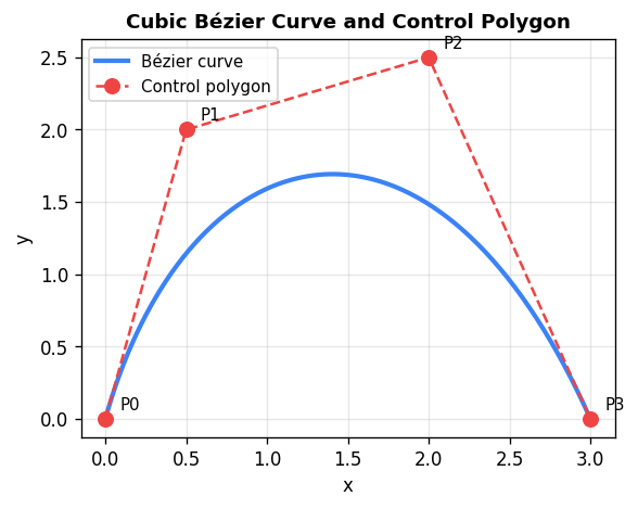
Bézier curves use control points rather than interpolation points. For control points \(\mathbf{p}_0, \ldots, \mathbf{p}_N\), the Bernstein basis polynomials of degree \(N\) are
\[ B_{i,N}(t) = \binom{N}{i} t^i (1-t)^{N-i}, \quad i = 0, \ldots, N, \]and the Bézier curve is \(\mathbf{P}(t) = \sum_{i=0}^{N} B_{i,N}(t)\,\mathbf{p}_i\) for \(t \in [0,1]\). Key properties: the curve interpolates the first and last control point (\(\mathbf{P}(0) = \mathbf{p}_0\), \(\mathbf{P}(1) = \mathbf{p}_N\)), the endpoint tangent directions are determined by the adjacent control points, and the curve lies entirely within the convex hull of its control points. Moving one control point produces a localized (though not entirely local) change.
Cubic B-splines provide fully local control: each curve segment \(B_i(u)\) depends on only four consecutive control points \(\mathbf{p}_{i-1}, \mathbf{p}_i, \mathbf{p}_{i+1}, \mathbf{p}_{i+2}\) via
\[ B_i(u) = b_{-1}\mathbf{p}_{i-1} + b_0\mathbf{p}_i + b_1\mathbf{p}_{i+1} + b_2\mathbf{p}_{i+2}, \]with blending functions \(b_{-1} = (1-u)^3/6\), \(b_0 = (2-3u^2+u^3)/3 + 1/6 - u^2/2\), etc. Adjacent curve pieces automatically share the same position, first derivative, and second derivative at their junction. Unlike Bézier curves, B-splines do not interpolate any control point (except in degenerate cases with repeated points).
Chapter 3: Planar Parametric Curves
A parametric curve in the plane is described by two continuous functions \(x(t)\) and \(y(t)\) of a common parameter \(t\), tracing out a directed path \(\mathbf{P}(t) = (x(t), y(t))\) for \(t \in [a, b]\). The parameter \(t\) need not have physical meaning — it is simply a coordinate along the curve.
The tangent direction at \(t = t_0\) is given by the first derivative vector \((x'(t_0), y'(t_0))\). A curve is smooth (in the mathematical sense) when all derivatives of \(x(t)\) and \(y(t)\) exist. A square described piecewise has corners at the transitions between pieces, reflecting the non-existence of derivatives there.
Interpolating Curve Data Parametrically
Given data points \((x_i, y_i)\), \(i = 1, \ldots, n\), we construct a parametric interpolant by:
- Assigning parameter values \(t_i\) to each data point — a natural choice uses arc-length parameterization: \[ t_{i+1} = t_i + \sqrt{(x_{i+1} - x_i)^2 + (y_{i+1} - y_i)^2}, \] which distributes the parameter values proportional to the chord lengths between points.
- Fitting a cubic spline through the data \((t_i, x_i)\) to obtain \(x_{cs}(t)\) and independently through \((t_i, y_i)\) to obtain \(y_{cs}(t)\).
The pair \((x_{cs}(t), y_{cs}(t))\) is a smooth parametric curve passing through all the data points. Arc-length parameterization (compared to the trivial \(t_i = i\)) produces significantly better visual results when points are irregularly spaced.
Application: Computer Representation of Handwriting
Script letters can be digitized by identifying their smooth curve segments, recording 8–16 data points per letter, assigning arc-length parameters, and fitting cubic splines to obtain smooth renderings. Closed curves (like the letter O) use periodic spline boundary conditions. This process produces the smooth “CS 370” logo appearing in the course notes, constructed entirely from parametric spline curves.
Chapter 4: Differential Equations
Introduction: Initial Value Problems
Many physical systems are described by an initial value problem (IVP):
\[ y'(t) = f(t, y(t)), \quad y(t_0) = y_0. \]Here \(f\) is the dynamics function and \((t_0, y_0)\) are the initial conditions. Classic examples:
- Exponential growth: \(y' = ay\) models an unconstrained population; the exact solution is \(y(t) = y_0 e^{a(t-t_0)}\).
- Logistic growth: \(y' = y(a - by)\) accounts for carrying capacity; the exact solution is \(y(t) = ay_0 e^{a(t-t_0)} / (by_0 e^{a(t-t_0)} + a - y_0 b)\).
- Complex ecological models: \(y' = y(a(t) - b(t)y^\alpha)\) with time-varying coefficients have no closed-form solution in general.
When no analytic solution exists, we seek a numerical solution: a sequence of approximate values \(y_0, y_1, \ldots, y_N\) at times \(t_0 < t_1 < \cdots < t_N\) such that \(y_n \approx y(t_n)\).
Higher-order ODEs and systems are handled by converting to first-order vector form. For example, the second-order equation \(y'' - ty' + ay = \sin t\) becomes
\[ \begin{pmatrix} y \\ z \end{pmatrix}' = \begin{pmatrix} z \\ tz - ay + \sin t \end{pmatrix}, \quad z = y'. \]Time-Stepping Methods
A general time-stepping method initializes \(y_0\), selects a candidate step size \(h_{\text{cand}}\), and iterates:
- Compute \(y_{n+1}\) and select \(h_n = t_{n+1} - t_n\) from \((t_n, y_n, h_{\text{cand}}, f)\).
- Advance \(t_{n+1} \leftarrow t_n + h_n\).
- Recompute \(h_{\text{cand}}\) for the next step.
Methods are classified as single-step (use only the current value) vs multi-step (use several past values), and as explicit (where \(y_{n+1}\) is computed directly) vs implicit (where \(y_{n+1}\) appears on both sides, requiring a nonlinear solve).
Forward Euler (Explicit, 1st Order)
The simplest scheme uses the tangent slope at \(t_n\) to extrapolate:
\[ y_{n+1} = y_n + h \cdot f(t_n, y_n). \]This is derived from the Taylor expansion \(y(t_{n+1}) = y(t_n) + hf(t_n, y(t_n)) + O(h^2)\). The local truncation error (error in one step assuming exact data) is \(O(h^2)\), giving global error \(O(h)\) — a first-order method.
Trapezoidal Rule (Implicit, 2nd Order)
By using the average slope at both endpoints:
\[ y_{n+1} = y_n + \frac{h}{2}\left[f(t_n, y_n) + f(t_{n+1}, y_{n+1})\right]. \]Since \(y_{n+1}\) appears on the right-hand side, this is an implicit method. Its local truncation error is \(O(h^3)\), giving global error \(O(h^2)\).
Modified Euler / Runge-Kutta 2 (Explicit, 2nd Order)
To avoid solving the implicit equation, use Forward Euler as a predictor then substitute into the trapezoidal rule as a corrector:
\[ k_1 = h f(t_n, y_n), \qquad k_2 = h f(t_n + h,\, y_n + k_1), \]\[ y_{n+1} = y_n + \frac{k_1 + k_2}{2}. \]This Modified Euler method (also called Improved Euler or RK2) achieves \(O(h^3)\) local truncation error and \(O(h^2)\) global error while remaining explicit.
Runge-Kutta 4 (RK4)
The most widely used single-step method computes four slope estimates per step:
\[ k_1 = hf(t_n, y_n),\quad k_2 = hf\!\left(t_n + \tfrac{h}{2}, y_n + \tfrac{k_1}{2}\right), \]\[ k_3 = hf\!\left(t_n + \tfrac{h}{2}, y_n + \tfrac{k_2}{2}\right),\quad k_4 = hf(t_n + h, y_n + k_3), \]\[ y_{n+1} = y_n + \frac{k_1}{6} + \frac{k_2}{3} + \frac{k_3}{3} + \frac{k_4}{6}. \]RK4 has \(O(h^5)\) local and \(O(h^4)\) global truncation error.
Adaptive Step Control: Runge-Kutta-Fehlberg (RK45)
Using a constant step size wastes computation where the solution changes slowly and is inaccurate where it changes rapidly. Adaptive methods estimate the local error at each step by comparing two methods of different orders. If \(y_{n+1}^*\) is a lower-order estimate and \(y_{n+1}\) a higher-order estimate, then
\[ \text{Local Error} \approx |y_{n+1}^* - y_{n+1}| \approx Ah^p \]and the optimal next step size is
\[ h_{\text{new}} = h_{\text{old}} \left(\frac{0.8 \cdot \text{tol}}{|y_{n+1}^* - y_{n+1}|}\right)^{1/p}. \]MATLAB’s ode45 implements the Dormand-Prince RK45 pair (orders 4 and 5), automatically adapting the step size to maintain a user-specified tolerance.
Global vs. Local Error
A method with local truncation error \(O(h^{p+1})\) achieves global error \(O(h^p)\). This is because if we integrate to a fixed time \(T\) with step size \(h\), the number of steps is \(O(1/h)\), and worst-case error accumulation gives global error \(\leq\) local error \(\times\) number of steps \(= O(h^{p+1}) \cdot O(1/h) = O(h^p)\).
A rigorous convergence proof for Forward Euler shows that if \(f\) satisfies a Lipschitz condition and \(|y''(t)| \leq M\), the global error satisfies
\[ |e_n| \leq \frac{Mh}{2K} e^{TK}, \]which goes to zero as \(h \to 0\). Including round-off error \(\delta\), the total error is bounded by \(\frac{1}{K}\!\left(\frac{M}{2}h + \frac{\delta}{h}\right)e^{TK}\), which is minimized at an optimal step size \(h_{\text{opt}} = \sqrt{2\delta/M}\) — taking finer steps eventually increases error due to accumulation of round-off.
Stability
Stability concerns the propagation of errors introduced in initial conditions. Test the method on the model equation \(y' = -\lambda y\), \(\lambda > 0\) (exact solution decays to zero). An algorithm is stable if initial perturbations remain bounded.
Forward Euler applied to the test equation: \(y_{n+1} = (1 - \lambda h) y_n\). The recursion converges iff \(|1 - \lambda h| < 1\), i.e., \(h < 2/\lambda\). Forward Euler is conditionally stable.
Backward Euler (implicit): \(y_{n+1} = y_n / (1 + \lambda h)\). The error decays as \(e_n = e_0/(1+\lambda h)^n \to 0\) for any \(h > 0\) and \(\lambda > 0\). Backward Euler is unconditionally stable.
Trapezoidal (Crank-Nicolson): Applied to the test equation, the amplification factor is \((1 - \frac{\lambda h}{2})/(1 + \frac{\lambda h}{2})\), which has magnitude strictly less than 1 for all \(h > 0\). Also unconditionally stable.
In general, implicit methods tend to have better stability than explicit methods, at the cost of requiring a nonlinear solve at each step.
Stiff Differential Equations
A problem is stiff if stability constraints force an explicit method to use step sizes much smaller than accuracy requires. Stiffness arises when the solution contains both fast-decaying transients and slow components of interest — common in chemical kinetics (reactions occurring on vastly different timescales) and multi-body dynamics. The symptom in practice: ode45 takes tiny steps even when the solution appears smooth. The cure: use stiff solvers like ode23s or ode15s, which use implicit methods with excellent stability properties.
Chapter 5: Discrete Fourier Transforms
Introduction to Fourier Analysis
Many real-world signals — prices, audio recordings, image intensities — are best understood by decomposing them into sinusoidal components of different frequencies. For instance, monthly orange-juice prices might have a strong annual cycle (seasonal supply), a ten-year cycle (climate), and noise at every other frequency. Fourier analysis converts a time-domain signal into a frequency-domain representation that makes these components visible.
Fourier Series
For a continuous periodic function \(f(t)\) with period \(T = 2\pi\), the Fourier series representation is
\[ f(t) = a_0 + \sum_{k=1}^\infty a_k \cos(kt) + \sum_{k=1}^\infty b_k \sin(kt). \]The coefficients are determined by orthogonality of the trig functions on \([0, 2\pi]\):
\[ a_0 = \frac{1}{2\pi}\int_0^{2\pi} f(t)\,dt, \qquad a_k = \frac{1}{\pi}\int_0^{2\pi} f(t)\cos(kt)\,dt, \qquad b_k = \frac{1}{\pi}\int_0^{2\pi} f(t)\sin(kt)\,dt. \]Using Euler’s formula \(e^{i\theta} = \cos\theta + i\sin\theta\), the series takes the compact complex form
\[ f(t) = \sum_{k=-\infty}^{\infty} c_k e^{ikt}, \qquad c_k = \frac{1}{2\pi}\int_0^{2\pi} f(t)e^{-ikt}\,dt. \]Each \(|c_k|\) measures how much “power” the frequency \(k/T\) contributes.
The Discrete Fourier Transform (DFT)
In practice, we have \(N\) sampled values \(f_0, f_1, \ldots, f_{N-1}\) at equally spaced times \(t_n = nT/N\). Let \(W = e^{2\pi i/N}\) be the \(N\)-th root of unity. The DFT pair is:
\[ \boxed{F_k = \frac{1}{N}\sum_{n=0}^{N-1} f_n W^{-nk}}, \qquad \boxed{f_n = \sum_{k=0}^{N-1} F_k W^{nk}}. \]The key orthogonality relation used in the derivation is:
\[ \sum_{j=0}^{N-1} W^{j(k-l)} = N\,\delta_{k,l}. \]The Fourier coefficients \(\{F_k\}\) form a doubly infinite periodic sequence with period \(N\): \(F_{k+N} = F_k\). For real-valued data, the conjugate symmetry property holds: \(F_k = \overline{F_{N-k}}\), so only \(N/2\) independent complex coefficients exist. The power spectrum \(\{|F_k|^2\}\) shows how energy is distributed across frequencies.
The Fast Fourier Transform (FFT)
Computing the DFT directly from the definition costs \(O(N^2)\) operations. The FFT exploits a divide-and-conquer strategy to reduce this to \(O(N \log_2 N)\), making transforms of millions of points feasible.
Assume \(N = 2^m\). Split the data into two half-length sequences:
\[ g_n = \frac{1}{2}(f_n + f_{n+N/2}), \qquad h_n = \frac{1}{2}(f_n - f_{n+N/2})W^{-n}, \quad n = 0, \ldots, N/2-1. \]Then the even-indexed and odd-indexed Fourier coefficients are:
\[ F_{2k} = \text{DFT}(g_n), \qquad F_{2k+1} = \text{DFT}(h_n), \]each of length \(N/2\). Applying this split recursively yields \(\log_2 N\) stages, each requiring \(O(N)\) operations — total \(O(N \log_2 N)\).
The butterfly diagram: Each stage of the FFT computes
\[ f_n' = \frac{1}{2}(f_n + f_{n+N/2}), \qquad f_{n+N/2}' = \frac{1}{2}(f_n - f_{n+N/2})W^{-n}. \]The data flow diagram resembles butterfly wings, giving the algorithm its name. After all \(\log_2 N\) butterfly stages, the output array contains \(F_0, \ldots, F_{N-1}\) in bit-reversed order: the output at index \(j\) contains \(F_p\) where \(p\) is obtained by reversing the binary digits of \(j\).
Image and Signal Compression
The DFT enables compression by exploiting the fact that most natural signals concentrate their energy in low-frequency components. The compression algorithm:
- Compute the DFT (or 2D DFT for images).
- Set Fourier coefficients below a threshold to zero.
- Reconstruct with the inverse DFT.
A 256×256 photo of Montreal can be compressed to 15% of its Fourier coefficients with minimal perceptible loss. This is the foundation of the JPEG standard, which applies 2D DCT (a variant of the DFT) to 8×8 or 16×16 pixel blocks.
Aliasing
When a continuous signal \(f(t)\) is sampled at \(N\) equally spaced points per period, the DFT coefficient \(F_l\) is not simply \(c_l\) (the true Fourier coefficient) but rather
\[ F_l = c_l + c_{l+N} + c_{l-N} + c_{l+2N} + \cdots \]If the signal contains frequencies above the Nyquist frequency \(N/(2T)\), those high-frequency components are aliased into lower frequencies, distorting the apparent spectrum. The cure: sample at a higher rate (\(\geq 2\times\) the highest frequency of interest), or low-pass filter before digitization.
The Correlation Function
Given two periodic signals \(y_i\) and \(z_i\), the cross-correlation
\[ \phi_n = \frac{1}{N}\sum_{i=0}^{N-1} y_{i+n} z_i \]measures how well \(z\) matches \(y\) when shifted by \(n\) positions. The maximum of \(\phi_n\) indicates the best-matching offset. A naive computation costs \(O(N^2)\), but using the convolution theorem:
\[ \Phi_k = Y_k \overline{Z_k}, \]followed by an inverse FFT recovers \(\phi_n\) in \(O(N \log N)\) operations.
The 2D DFT
For a gray-scale image array \(f_{n,j}\), \(n = 0, \ldots, N-1\), \(j = 0, \ldots, M-1\):
\[ F_{k,l} = \frac{1}{NM}\sum_{n=0}^{N-1}\sum_{j=0}^{M-1} f_{n,j}\, W_N^{-nk}\, W_M^{-jl}. \]This can be computed as a sequence of 1D FFTs: first apply 1D FFTs of length \(M\) to each row, then 1D FFTs of length \(N\) to each column. Total cost: \(O(NM(\log_2 M + \log_2 N))\).
Chapter 6: Numerical Linear Algebra
Solving Linear Systems via LU Factorization
Given an \(n \times n\) matrix \(A\) and right-hand side vector \(\mathbf{b}\), we want to solve \(A\mathbf{x} = \mathbf{b}\). The standard computational approach factors \(A = LU\) where \(L\) is unit lower triangular (1s on diagonal) and \(U\) is upper triangular, then solves the two easy triangular systems:
- Forward solve: \(L\mathbf{z} = \mathbf{b}\) (substitute forward: \(z_i = b_i - \sum_{j \lt i} l_{ij} z_j\)).
- Back solve: \(U\mathbf{x} = \mathbf{z}\) (substitute backward: \(x_i = (z_i - \sum_{j>i} u_{ij} x_j)/u_{ii}\)).
LU factorization algorithm (Gaussian elimination, storing multipliers):
For k = 1, ..., n
  For i = k+1, ..., n
    mult = a[i,k] / a[k,k]
    a[i,k] = mult          // store L below diagonal
    For j = k+1, ..., n
      a[i,j] -= mult * a[k,j]   // update U above diagonal
After factorization, the lower part of the (modified) array stores \(L\) and the upper part stores \(U\). The key advantage: once \(A = LU\) is computed (at cost \(O(n^3/3)\) flops), each new right-hand side requires only \(O(n^2)\) for the two triangular solves. Computing \(A^{-1}\) follows by solving \(n\) systems with right-hand sides equal to the columns of the identity.
Gaussian Elimination ≡ Matrix Factorization
Gaussian elimination can be viewed as multiplying \(A\) on the left by a sequence of elementary lower triangular matrices \(M^{(k)}\) that zero out entries below the diagonal in column \(k\). Each \(M^{(k)}\) differs from the identity only in column \(k\) below the diagonal. The product \(M^{(n-1)} \cdots M^{(1)} A = U\) is upper triangular, so \(A = (M^{(1)})^{-1} \cdots (M^{(n-1)})^{-1} U = LU\).
Pivoting: When the pivot element \(a_{kk}\) is zero (or small), numerical instability occurs. Partial pivoting reorders equations (rows) to make the largest element in the current column the pivot, encoded by a permutation matrix \(P\): the factorization becomes \(PA = LU\).
Condition Numbers and Norms
The condition number of a matrix measures how sensitive the solution of \(A\mathbf{x} = \mathbf{b}\) is to perturbations in \(\mathbf{b}\) (or \(A\)). For an invertible matrix \(A\),
\[ \kappa(A) = \|A\|\cdot\|A^{-1}\|. \]The vector \(p\)-norm is \(\|\mathbf{x}\|_p = \left(\sum |x_i|^p\right)^{1/p}\); the matrix norm induced by the vector norm satisfies \(\|A\mathbf{x}\| \leq \|A\|\cdot\|\mathbf{x}\|\).
If \(A\hat{\mathbf{x}} = \mathbf{b}\) is the computed solution, the residual is \(\mathbf{r} = \mathbf{b} - A\hat{\mathbf{x}}\). The relative error in the solution is bounded by
\[ \frac{\|\hat{\mathbf{x}} - \mathbf{x}\|}{\|\mathbf{x}\|} \leq \kappa(A) \cdot \frac{\|\mathbf{r}\|}{\|\mathbf{b}\|}. \]A small residual does not guarantee a small error if \(\kappa(A)\) is large — a well-known pitfall with ill-conditioned matrices.
Chapter 7: Google PageRank
Introduction: The Web as a Random Walk
The PageRank algorithm, the basis of Google’s original search ranking, models a user (“random surfer”) who randomly follows hyperlinks. A page’s importance is proportional to the probability that the surfer is visiting it at a random time. More important pages are those linked to by many other important pages.
The Transition Matrix
Let the web contain \(R\) pages. Define an \(R \times R\) matrix \(P\) where \(P_{ij}\) is the probability of moving from page \(j\) to page \(i\) — equal to \(1/(\text{number of links on page } j)\) if page \(j\) links to page \(i\), and 0 otherwise. Two problems arise:
- Dead-end pages (no outgoing links): the surfer gets stuck. Fix: teleport to a random page with probability 1.
- Cycling pages (the surfer gets trapped in a cluster): the algorithm may not converge. Fix: with probability \(1-\alpha\), teleport to a random page.
The Google matrix \(M\) is constructed as follows. Let \(\mathbf{d}\) mark dead-end pages (\(d_j = 1\) if page \(j\) has no out-links), and \(\mathbf{e} = (1,1,\ldots,1)^T\). First form
\[ Q = P + \frac{1}{R}\mathbf{e}\mathbf{d}^T. \]Then incorporate the teleportation parameter \(\alpha \in (0,1)\) (typically \(\alpha = 0.85\)):
\[ M = \alpha Q + \frac{1-\alpha}{R}\mathbf{e}\mathbf{e}^T. \]Every entry of \(M\) is positive and each column sums to 1 — \(M\) is a positive Markov (column-stochastic) matrix.
The PageRank Algorithm
The PageRank vector \(\mathbf{p}^\infty\) is the unique probability vector satisfying \(M\mathbf{p}^\infty = \mathbf{p}^\infty\) — the stationary distribution of the Markov chain. It is computed by the power method:
\[ \mathbf{p}^0 = \frac{\mathbf{e}}{R}, \qquad \mathbf{p}^{k+1} = M\mathbf{p}^k, \qquad \text{until } \max_i |p_i^{k+1} - p_i^k| < \text{tol}. \]Pages are then ranked by the components of \(\mathbf{p}^\infty\).
Convergence Analysis
Since \(M\) is a positive Markov matrix, it has \(\lambda_1 = 1\) as its dominant eigenvalue (largest in magnitude), with a unique eigenvector. All other eigenvalues satisfy \(|\lambda_l| < 1\). Writing the initial vector in the eigenbasis:
\[ M^k \mathbf{p}^0 = c_1 \mathbf{x}_1 + \sum_{l \geq 2} c_l \lambda_l^k \mathbf{x}_l \xrightarrow{k \to \infty} c_1 \mathbf{x}_1 = \mathbf{p}^\infty, \]so the power method converges for any starting probability vector. The rate of convergence is governed by the second-largest eigenvalue: one can show \(|\lambda_2| \approx \alpha\). For \(\alpha = 0.85\), approximately \(114\) iterations suffice to achieve \(10^{-8}\) accuracy.
Practical efficiency: Although \(M\) is a dense \(R \times R\) matrix (with billions of pages, this is enormous), the multiplication \(M\mathbf{p}^k\) can be performed in \(O(R)\) operations by exploiting the sparse structure of \(P\):
\[ M\mathbf{p}^k = \alpha\left(P + \frac{1}{R}\mathbf{e}\mathbf{d}^T\right)\mathbf{p}^k + \frac{1-\alpha}{R}\mathbf{e}. \]Since \(P\) is sparse, \(P\mathbf{p}^k\) is computed efficiently, and the remaining terms involve cheap vector additions. The ranking vector is precomputed and updated periodically (every few weeks), separate from the query-time keyword matching.
Chapter 8: Least Squares Problems
The Least Squares Setting
Many fitting problems involve more equations than unknowns: given an \(m \times n\) matrix \(A\) with \(m > n\) (overdetermined) and a vector \(\mathbf{b} \in \mathbb{R}^m\), find \(\mathbf{x} \in \mathbb{R}^n\) that makes \(A\mathbf{x}\) as close to \(\mathbf{b}\) as possible. An exact solution \(A\mathbf{x} = \mathbf{b}\) will generically not exist when \(m > n\).
Motivating example: An overexposed photograph can be modeled as the true image plus a linear combination of known artifact patterns: \(\mathbf{y} = A\boldsymbol{\beta} + \boldsymbol{\epsilon}\) where \(\mathbf{y}\) is the observed (corrupted) image vectorized into a long column, \(A = [\mathbf{a}_1 | \mathbf{a}_2 | \mathbf{a}_3]\) contains the vectorized artifact patterns, \(\boldsymbol{\beta}\) are the unknown artifact strengths, and \(\boldsymbol{\epsilon}\) is the uncorrupted image. We want \(\boldsymbol{\beta}\) that best removes the artifacts.
The Normal Equations
The total squared error (or sum of squared residuals) is
\[ E(\mathbf{x}) = \|A\mathbf{x} - \mathbf{b}\|_2^2 = (A\mathbf{x} - \mathbf{b})^T(A\mathbf{x} - \mathbf{b}). \]Minimizing \(E(\mathbf{x})\) by differentiating with respect to each \(x_l\) and setting to zero yields the normal equations:
\[ A^T A\,\mathbf{x} = A^T \mathbf{b}. \]When the columns of \(A\) are linearly independent (\(A\) has full column rank), \(A^T A\) is symmetric positive definite and hence nonsingular. The least squares solution is then uniquely \(\mathbf{x} = (A^T A)^{-1} A^T \mathbf{b}\).
Conditioning caveat: If \(\kappa(A)\) is the condition number of \(A\), then \(\kappa(A^T A) = \kappa(A)^2\). Solving the normal equations via Gaussian elimination on \(A^T A\) squares the condition number, making the computation significantly less accurate than alternatives.
The QR Decomposition
A more numerically stable approach uses Givens rotations to reduce \(A\) to upper triangular form without squaring the condition number. A Givens rotation matrix \(Q\) differs from the identity in a \(2 \times 2\) block:
\[ Q_{ii} = c, \quad Q_{jj} = c, \quad Q_{ij} = s, \quad Q_{ji} = -s, \quad c^2 + s^2 = 1. \]Multiplying a vector by \(Q\) affects only rows \(i\) and \(j\):
\[ [Qx]_i = cx_i + sx_j, \qquad [Qx]_j = -sx_i + cx_j. \]Choosing \(c = x_i/\sqrt{x_i^2 + x_j^2}\) and \(s = x_j/\sqrt{x_i^2 + x_j^2}\) sets \([Qx]_j = 0\). Since \(Q\) is orthogonal (\(Q^T Q = I\)), multiplication by \(Q\) preserves vector length: \(\|Q^T\mathbf{r}\|_2 = \|\mathbf{r}\|_2\).
Applying a sequence of Givens rotations \(Q^{(1)}, Q^{(2)}, \ldots\) to \(A\) zeros out entries below the diagonal, producing the QR decomposition \(A = QR\) where \(Q\) is orthogonal and \(R\) is upper triangular. Since orthogonal transformations preserve the 2-norm:
\[ \|A\mathbf{x} - \mathbf{b}\|_2 = \|Q^T(A\mathbf{x} - \mathbf{b})\|_2 = \|R\mathbf{x} - Q^T\mathbf{b}\|_2, \]and the minimum is achieved by solving the square upper triangular system \(R\mathbf{x} = (Q^T\mathbf{b})_{1:n}\) (the first \(n\) components). This approach is more stable because the condition number of \(R\) equals \(\kappa(A)\) rather than \(\kappa(A)^2\).
