Notes by TC Fraser, Fall 2016. Supplemented from Barbara Ryden, Introduction to Cosmology (2nd ed.).

---

Chapter 1: The Foundations of Modern Cosmology

Section 1.1: The Cosmological Principle and the Observable Universe

The Cosmological Principle

The starting point of modern cosmology is an audacious claim about our place in the universe. The Cosmological Principle asserts that the universe is both homogeneous — the same everywhere in space — and isotropic — the same in every direction. These are not obvious facts. The night sky is clearly patchy: there are dense star clusters and vast dark voids, conspicuous bright galaxies and stretches of apparent emptiness. Yet when we average over sufficiently large scales — roughly 100 Mpc or more — the universe does appear to be uniform. Deep galaxy surveys confirm that, on scales larger than the spacing between superclusters, the distribution of matter smooths out to a nearly constant density, and observations of the cosmic microwave background reveal that the sky is uniform in temperature to one part in \(10^5\).

The Cosmological Principle is more than a convenience; it is a philosophical statement. It rules out the possibility that we occupy a special location in the cosmos — a position with deep roots in the Copernican revolution. If the universe is homogeneous and isotropic, then every observer everywhere sees the same large-scale structure, the same expansion rate, the same cosmic history. This symmetry dramatically restricts the possible geometries of the universe and the form of the metric describing spacetime, as we will see when we derive the Friedmann–Robertson–Walker metric.

Olbers’ Paradox

A deceptively simple question reveals a profound truth about cosmology: why is the night sky dark? In an infinite, eternal, static universe uniformly filled with stars, every line of sight would eventually terminate on a stellar surface, and the night sky would blaze with the uniform brightness of a stellar surface — hotter and brighter than the Sun. The fact that the sky is dark at night, sometimes called Olbers’ Paradox, therefore rules out a static infinite universe.

There are two resolutions consistent with observation. Either the universe has finite age, so that light from sufficiently distant stars has not had time to reach us, or the universe is expanding, so that distant light is redshifted to such low energies that it no longer contributes significantly to the optical night sky. In our universe, both effects operate simultaneously. The cosmic microwave background is the faint relic of a time when the sky truly was uniformly bright — but at temperatures corresponding to infrared and microwave photons invisible to the naked eye.

Cosmic Structures

The universe is organized hierarchically. Planets orbit stars, which gather into galaxies containing \(10^{10}\) to \(10^{12}\) stars spanning tens to hundreds of kiloparsecs. Galaxies cluster gravitationally into galaxy groups and galaxy clusters containing hundreds to thousands of galaxies spread over a few megaparsecs. Clusters in turn form part of superclusters and the larger cosmic web — a network of filaments and walls surrounding vast empty voids. The typical void diameter is roughly 30–50 Mpc, and the superclusters span up to 100 Mpc. Beyond this scale, the universe is homogeneous to good approximation, and the Cosmological Principle applies.

The Discovery of Expansion and the CMB

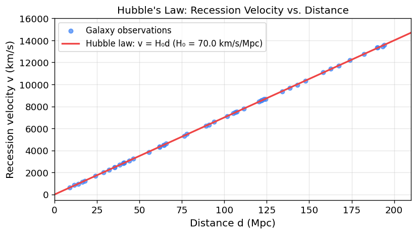
Edwin Hubble’s 1929 observation that galaxies recede from us at velocities proportional to their distances was among the most consequential measurements in the history of astronomy. Hubble’s Law states:

\[v = H_0 \, d,\]

where \(v\) is the recession velocity, \(d\) is the proper distance, and \(H_0\) is the Hubble constant, measured today as \(H_0 \approx 68 \text{ km s}^{-1} \text{ Mpc}^{-1}\).

The Hubble constant sets a natural timescale — the Hubble time:

\[t_H = \frac{1}{H_0} \approx 14 \text{ Gyr},\]

which gives an order-of-magnitude estimate of the age of the universe. The recession of galaxies implies that the universe was once much denser. Extrapolating backward in time leads to the Big Bang — a hot, dense initial state from which the universe has been expanding and cooling ever since.

The most compelling evidence for the Hot Big Bang is the cosmic microwave background (CMB), discovered serendipitously in 1965 by Arno Penzias and Robert Wilson at Bell Laboratories. They detected an isotropic microwave signal at a temperature \(T_0 = 2.725 \text{ K}\) coming from every direction in the sky. Robert Dicke and his Princeton group recognized this as the cooled relic radiation of the primordial fireball — photons that last scattered off matter when the universe was about 380,000 years old and have been redshifting freely ever since.

---

Section 1.2: Newtonian Cosmology and the Friedmann Equation

Co-moving Coordinates and the Scale Factor

To describe an expanding universe, we introduce co-moving coordinates \(\mathbf{x}\), which follow the average motion of matter. The physical position of a point is related to its co-moving coordinate by:

\[\mathbf{r} = a(t) \, \mathbf{x},\]

where \(a(t)\) is the scale factor, normalized so that \(a(t_0) = 1\) today. As the universe expands, \(a\) increases. The physical velocity of a particle has two contributions: the Hubble flow and the peculiar velocity. For a co-moving particle (no peculiar velocity):

\[\dot{\mathbf{r}} = \dot{a} \mathbf{x} = \frac{\dot{a}}{a} \mathbf{r} = H(t) \mathbf{r},\]

which is precisely Hubble’s Law with the Hubble parameter \(H(t) = \dot{a}/a\). At the present epoch, \(H(t_0) = H_0\).

The Friedmann Equation from Newtonian Gravity

Despite being a fundamentally general-relativistic result, the Friedmann equation can be derived from Newtonian mechanics for a spatially flat universe, using the shell theorem: the gravitational force on a thin shell depends only on the mass enclosed. Consider a test mass \(m\) at the edge of a sphere of radius \(r = a(t)x\) containing homogeneous matter of density \(\rho(t)\). The total mass enclosed is:

\[M = \frac{4}{3} \pi r^3 \rho.\]

The energy of the test mass (per unit mass) is:

\[E = \frac{1}{2}\dot{r}^2 - \frac{GM}{r} = \frac{1}{2}\dot{r}^2 - \frac{4\pi G \rho r^2}{6}.\]

Since \(\dot{r} = Hx \cdot a = Hr\) for a co-moving particle, substituting:

\[E = \frac{1}{2}H^2 r^2 - \frac{4\pi G \rho r^2}{3}.\]

Setting \(E = -\frac{kc^2 x^2}{2}\) (a constant of integration, where \(k\) is the spatial curvature parameter) and dividing by \(r^2/2\):

\[\boxed{H^2 = \frac{8\pi G}{3}\rho - \frac{kc^2}{a^2}.}\]

This is the Friedmann equation. The curvature parameter \(k = -1, 0, +1\) corresponds to open, flat, and closed universes respectively. Physically, \(E < 0\) (closed), \(E = 0\) (flat), and \(E > 0\) (open) universes are analogous to bound, marginally bound, and unbound orbits.

Conservation of Energy: the Continuity Equation

Energy conservation in an expanding universe, or equivalently the first law of thermodynamics applied to a co-moving volume, gives the continuity equation (also called the fluid equation):

\[\dot{\rho} = -3H\left(\rho + \frac{P}{c^2}\right),\]

where \(P\) is the pressure of the cosmic fluid. The factor of 3 arises because the volume expands in all three dimensions. The term \(P/c^2\) reflects the relativistic energy content of pressure — in a rapidly expanding universe, pressure does work and contributes to the energy budget.

The Acceleration Equation

Differentiating the Friedmann equation with respect to time and using the continuity equation yields the acceleration equation:

\[\frac{\ddot{a}}{a} = -\frac{4\pi G}{3}\left(\rho + \frac{3P}{c^2}\right).\]

This is crucial: both energy density \(\rho c^2\) and pressure \(P\) contribute to the gravitational deceleration of the expansion. For ordinary matter with \(P > 0\), gravity decelerates the expansion. Only when \(P < -\rho c^2/3\) does the expansion accelerate — a condition satisfied by the cosmological constant (dark energy).

---

Section 1.3: The Friedmann–Robertson–Walker Metric

Spatial Geometry of the Universe

The Cosmological Principle constrains the spatial geometry of the universe to one of three homogeneous, isotropic possibilities. In spherical polar coordinates, the spatial metric is:

\[d\ell^2 = \frac{dr^2}{1 - kr^2} + r^2\left(d\theta^2 + \sin^2\theta\, d\phi^2\right),\]

where \(k = -1\) (hyperbolic/open), \(k = 0\) (Euclidean/flat), or \(k = +1\) (spherical/closed). Note that this is the metric on the spatial hypersurface at a fixed time — it describes the intrinsic geometry of space, not spacetime.

The Full FRW Metric

Including the time dimension and the expansion of space, the Friedmann–Robertson–Walker (FRW) metric is:

\[ds^2 = -c^2 dt^2 + a^2(t)\left[\frac{dr^2}{1-kr^2} + r^2 d\Omega^2\right],\]

where \(d\Omega^2 = d\theta^2 + \sin^2\theta\, d\phi^2\) is the solid angle element. This metric encodes the entire spacetime geometry of a homogeneous, isotropic universe in a single function — the scale factor \(a(t)\). The coordinate \(r\) is the co-moving radial coordinate; the physical radial distance at cosmic time \(t\) is \(a(t)r\) (for a flat universe).

General Relativity: Principles and Einstein’s Equations

Newtonian gravity fails in strong gravitational fields and at relativistic velocities. General relativity (GR) replaces Newton’s theory with a geometric description of gravity. The two key principles are:

1. Equivalence Principle: The laws of physics are the same in all freely falling (inertial) reference frames. Locally, a freely falling observer cannot distinguish between gravity and acceleration. This identifies gravity as spacetime curvature.
2. Geodesic equation: Free particles (and photons) follow geodesics — the straightest possible paths through curved spacetime. For massive particles: \(\ddot{x}^\mu + \Gamma^\mu_{\alpha\beta}\dot{x}^\alpha \dot{x}^\beta = 0\), where \(\Gamma^\mu_{\alpha\beta}\) are the Christoffel symbols encoding the curvature.

The field equations of GR relate spacetime curvature to the energy-momentum content:

\[G_{\mu\nu} = \frac{8\pi G}{c^4} T_{\mu\nu} + \Lambda g_{\mu\nu},\]

where \(G_{\mu\nu} = R_{\mu\nu} - \frac{1}{2}Rg_{\mu\nu}\) is the Einstein tensor (encoding curvature), \(T_{\mu\nu}\) is the stress-energy tensor (encoding matter and energy), \(g_{\mu\nu}\) is the metric, and \(\Lambda\) is the cosmological constant. The cosmological constant, which Einstein introduced and later called his “greatest blunder,” turns out to be necessary to explain the observed accelerated expansion.

The Cosmological Equations

For a perfect fluid with energy density \(\rho c^2\) and pressure \(P\), the stress-energy tensor is \(T_{\mu\nu} = (\rho + P/c^2)u_\mu u_\nu + Pg_{\mu\nu}\), where \(u^\mu\) is the four-velocity of the fluid. Substituting the FRW metric and this stress-energy tensor into Einstein’s equations yields the complete set of cosmological equations:

Only two of these three equations are independent; the third follows from the other two combined with energy conservation. Together, they govern the entire dynamical history of the universe.

Cosmological Redshift

A photon traveling through an expanding universe is stretched along with the fabric of space. Consider a photon emitted at time \(t_e\) with wavelength \(\lambda_e\) and received at time \(t_0\) with wavelength \(\lambda_0\). Since the physical scale has grown by a factor \(a(t_0)/a(t_e) = 1/a(t_e)\) (with \(a_0 = 1\)), the wavelength is stretched by the same factor. The cosmological redshift \(z\) is defined by:

\[1 + z = \frac{\lambda_0}{\lambda_e} = \frac{a_0}{a(t_e)} = \frac{1}{a(t_e)}.\]

Redshift is thus a direct measure of the scale factor at the time of emission. A photon received from redshift \(z = 1\) was emitted when the universe was half its current size; the CMB photons at \(z \approx 1100\) were emitted when the universe was about a thousand times smaller than today.

---

Chapter 2: Observational Cosmology

Section 2.1: Cosmic Eras — Equations of State and Scale Factor Solutions

Equations of State

The behavior of the scale factor depends on what the universe is made of. Each component is characterized by its equation of state parameter \(w\), defined by \(P = w\rho c^2\). The continuity equation integrates to give:

\[\rho \propto a^{-3(1+w)}.\]

Matter (dust): Non-relativistic matter has negligible pressure, \(w = 0\), \(P = 0\). The density dilutes with the expanding volume:

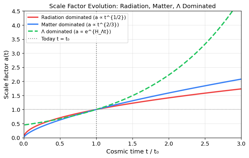
\[\rho_m \propto a^{-3}.\]

In a matter-dominated flat universe, Friedmann’s equation gives \(a \propto t^{2/3}\), and \(H = 2/(3t)\).

Radiation: For a relativistic gas of photons, \(P = \rho c^2/3\), so \(w = 1/3\). The energy density redshifts faster than matter — not only does the number of photons per unit volume dilute as \(a^{-3}\), but each photon also loses energy to the cosmological redshift:

\[\rho_r \propto a^{-4}.\]

In a radiation-dominated flat universe, \(a \propto t^{1/2}\) and \(H = 1/(2t)\).

Dark Energy (Cosmological Constant): The cosmological constant acts as a fluid with \(w = -1\), i.e., \(P_\Lambda = -\rho_\Lambda c^2\). The continuity equation then gives \(\dot{\rho}_\Lambda = 0\) — a constant energy density. From the acceleration equation, this constant energy density produces an exponentially accelerating expansion:

\[a \propto e^{H_\Lambda t}, \quad H_\Lambda = \sqrt{\frac{\Lambda c^2}{3}} = \text{const}.\]

Curvature: The curvature term in the Friedmann equation behaves as an effective fluid with \(w = -1/3\), \(\rho_k \propto a^{-2}\).

The Sequence of Cosmic Eras

The total energy density of the universe is a sum of all components. Which component dominates the dynamics changes over time. Since \(\rho_r \propto a^{-4}\) and \(\rho_m \propto a^{-3}\), radiation dominates at small \(a\) (early times) and matter dominates later. Dark energy has a constant density and eventually comes to dominate at late times.

The transitions between eras are characterized by equality redshifts:

• Radiation–matter equality: \(\rho_r = \rho_m\) at \(z_{eq} \approx 3400\) (when the universe was about 50,000 years old). Before this epoch, the universe was radiation-dominated.
• Matter–dark energy equality: \(\rho_m = \rho_\Lambda\) at \(z \approx 0.3\), corresponding to a lookback time of a few billion years. Since then, the universe has been dark-energy dominated and accelerating.

This sequence — radiation → matter → dark energy — defines the broad thermal and dynamical history of the cosmos.

---

Section 2.2: Distances and the Discovery of Dark Energy

The Density Parameter

The critical density is the density for which a flat universe (\(k = 0\)) satisfies the Friedmann equation:

\[\rho_c = \frac{3H^2}{8\pi G}.\]

At the present epoch, \(\rho_{c,0} = 3H_0^2/(8\pi G) \approx 1.28 \times 10^{11} M_\odot \text{ Mpc}^{-3} \approx 9.5 \times 10^{-27} \text{ kg m}^{-3}\). The density parameter for each component is:

\[\Omega_i = \frac{\rho_i}{\rho_c}.\]

The Friedmann equation in terms of density parameters is:

\[\frac{H^2}{H_0^2} = \Omega_{m,0}\,(1+z)^3 + \Omega_{r,0}\,(1+z)^4 + \Omega_{\Lambda,0} + \Omega_{k,0}\,(1+z)^2,\]

where the curvature density parameter is \(\Omega_{k,0} = 1 - \Omega_{m,0} - \Omega_{r,0} - \Omega_{\Lambda,0}\), and vanishes for a flat universe. Current observations give \(\Omega_{m,0} \approx 0.31\), \(\Omega_{\Lambda,0} \approx 0.69\), and \(\Omega_{k,0} \approx 0\).

The Deceleration Parameter

The deceleration parameter quantifies whether the expansion is speeding up or slowing down:

\[q \equiv -\frac{\ddot{a} \, a}{\dot{a}^2} = \frac{\Omega_m}{2} + \Omega_r - \Omega_\Lambda,\]

where the last equality holds approximately in the matter + dark energy era. A universe with \(q > 0\) decelerates; \(q < 0\) means accelerated expansion. The universe transitions from deceleration to acceleration when \(\Omega_\Lambda > \Omega_m/2\), which in our universe occurred at \(z \approx 0.7\).

Standard Candles and the Discovery of Cosmic Acceleration

A standard candle is any object whose intrinsic luminosity \(L\) is known. By measuring the observed flux \(f\) and using \(f = L/(4\pi d_L^2)\), one can infer the luminosity distance \(d_L\). If the source is also at a known redshift \(z\), one obtains a point on the \(d_L\)-versus-\(z\) Hubble diagram, which is sensitive to the cosmological model.

Type Ia supernovae are the premier standard candles at cosmological distances. A Type Ia supernova begins as a white dwarf accreting mass from a companion. When the white dwarf approaches the Chandrasekhar mass \(M_{Ch} \approx 1.4 M_\odot\), electron degeneracy pressure can no longer support it, and a runaway nuclear fusion reaction destroys the entire star, producing a peak luminosity of \(L \approx 4 \times 10^9 L_\odot\) — bright enough to be seen across the universe at \(z \sim 1\). The peak luminosity correlates tightly with the shape of the light curve (broader light curve → more luminous), allowing calibration to about 5% precision.

In 1998–1999, two independent teams — the Supernova Cosmology Project (Perlmutter et al.) and the High-Z Supernova Search Team (Schmidt, Riess et al.) — measured Type Ia supernovae at \(z > 0.3\) and found them systematically fainter than expected in a matter-only decelerating universe. The supernovae were more distant than a flat matter-only universe would predict, implying that the expansion has been accelerating. This discovery, recognized with the 2011 Nobel Prize in Physics, requires \(\Omega_\Lambda > 0\) and \(q_0 < 0\). Combined with CMB flatness constraints, the data are consistent with the Benchmark Model: \(\Omega_{m,0} \approx 0.3\), \(\Omega_{\Lambda,0} \approx 0.7\).

The Cosmological Constant Problem

The dark energy density required to explain cosmic acceleration is:

\[\rho_\Lambda c^2 = \frac{\Lambda c^4}{8\pi G} \approx 3.8 \times 10^{-10} \text{ J m}^{-3} \approx (2.4 \times 10^{-3} \text{ eV})^4.\]

Quantum field theory predicts that vacuum fluctuations should contribute to the energy density of empty space. The natural scale for the vacuum energy density is set by the cutoff of quantum field theory, which is at least the electroweak scale \(\sim 100\) GeV or possibly the Planck scale \(\sim 10^{18}\) GeV. The theoretical prediction exceeds the observed dark energy density by a factor of at least \(10^{56}\) and possibly as much as \(10^{120}\). This enormous discrepancy, the cosmological constant problem, remains one of the deepest unsolved problems in physics.

The Age of the Universe

The age of the universe is:

\[t_0 = \int_0^1 \frac{da}{a H(a)} = \frac{1}{H_0}\int_0^1 \frac{da}{a\sqrt{\Omega_{m,0} a^{-3} + \Omega_{\Lambda,0}}}.\]

In a pure matter-dominated flat universe (\(\Omega_m = 1\)), this gives \(t_0 = 2/(3H_0) \approx 9 \text{ Gyr}\). This was historically troublesome because observations of globular clusters put their ages at \(12\)–\(14\) Gyr — older than the universe itself, the age crisis. Including dark energy resolves the problem: with \(\Omega_{m,0} \approx 0.31\), \(\Omega_{\Lambda,0} \approx 0.69\), the integral gives \(t_0 \approx 13.8 \text{ Gyr}\), comfortably older than any observed stellar population.

---

Section 2.3: Geodesics and Cosmological Distances

Null Geodesics in the FRW Spacetime

Light travels along null geodesics, for which \(ds^2 = 0\). For radial photons in the FRW metric:

\[0 = -c^2 dt^2 + a^2(t)\frac{dr^2}{1-kr^2}.\]

For a flat universe (\(k = 0\)):

\[\frac{c\, dt}{a(t)} = dr.\]

This can be integrated to give the co-moving distance to a source at redshift \(z\):

\[r(z) = c\int_0^z \frac{dz'}{H(z')} = \frac{c}{H_0}\int_0^z \frac{dz'}{\sqrt{\Omega_{m,0}(1+z')^3 + \Omega_{r,0}(1+z')^4 + \Omega_{\Lambda,0}}}.\]

The co-moving distance is the distance measured in today’s coordinate system, independent of when the observation was made. It is the most natural distance measure for cosmology.

Luminosity Distance and Angular Diameter Distance

The luminosity distance \(d_L\) is defined so that \(f = L/(4\pi d_L^2)\). It accounts for two additional factors that dilute the flux compared to flat, static space: the redshifting of photon energies by \((1+z)^{-1}\), and the reduction in photon arrival rate by another \((1+z)^{-1}\). Together:

\[d_L = a_0 \, r(z) \, (1+z) = r(z)(1+z).\]

The angular diameter distance \(d_A\) is defined so that the observed angular size \(\delta\theta\) of an object of physical size \(\ell\) satisfies \(\delta\theta = \ell / d_A\):

\[d_A = \frac{r(z)}{1+z} = \frac{d_L}{(1+z)^2}.\]

Note that \(d_A\) is smaller than the co-moving distance — a remarkable consequence of expansion is that objects can actually appear larger as they move farther away (for \(z \gtrsim 1\)). The Etherington relation \(d_L = (1+z)^2 d_A\) is a model-independent consequence of general relativity and the Cosmological Principle.

Proper Distance and the Horizon

The proper distance at time \(t\) to a source at redshift \(z\) is \(d_p = a(t) r(z)\). The particle horizon — the maximum distance from which light could have reached us in the age of the universe — is:

\[d_H = a_0 \int_0^{t_0} \frac{c\, dt'}{a(t')}.\]

For a flat matter-dominated universe, this gives \(d_H = 3ct_0\) — about 46 Gpc in our universe. The existence of a finite particle horizon is central to the horizon problem of inflation.

---

Section 2.4: Dark Matter — Evidence and Probes

The Visible Universe

Before confronting the mystery of dark matter, it is instructive to take stock of what can be seen. Surveys of galaxies in the local universe reveal a luminosity density in the visual band of \(\Psi_V \approx 1.1 \times 10^8 L_{\odot,V} \text{ Mpc}^{-3}\). Converting to a mass density using the average mass-to-light ratio \(\langle M/L_V \rangle \approx 4 M_\odot/L_{\odot,V}\):

\[\rho_{\star,0} = \langle M/L_V \rangle \Psi_V \approx 4 \times 10^8 M_\odot \text{ Mpc}^{-3},\]

giving a density parameter in stars of:

\[\Omega_{\star,0} = \frac{\rho_{\star,0}}{\rho_{c,0}} \approx 0.003.\]

Even when stellar remnants (white dwarfs, neutron stars, black holes) and substellar objects (brown dwarfs) are included, \(\Omega_{\star,0} < 0.005\). Stars contribute at most 0.5% of the critical density. The night sky, for all its glory, is a minority of the baryonic matter in the universe, and baryons themselves are a minority of all matter.

Rotation Curves of Spiral Galaxies

The most direct evidence for dark matter in galaxies comes from measuring the orbital velocities of stars and gas as a function of radius. For a star on a circular orbit at radius \(R\) from the galactic center, Newton’s law gives:

\[\frac{v^2}{R} = \frac{GM(R)}{R^2} \implies v = \sqrt{\frac{GM(R)}{R}},\]

where \(M(R)\) is the total mass within radius \(R\). The surface brightness of a spiral galaxy falls off exponentially with scale length \(R_s\): \(I(R) = I(0)\exp(-R/R_s)\). Beyond a few scale lengths, almost all the stellar mass is concentrated within a central sphere, so if stars were the only matter, \(M(R)\) would be roughly constant at large \(R\) and \(v \propto R^{-1/2}\) — Keplerian rotation.

Instead, observations reveal flat rotation curves extending to many times the optical disk. Vera Rubin and Kent Ford (1970) measured the rotation curve of M31 out to \(R = 24 \text{ kpc} = 4R_s\) and found no Keplerian decline. Extended HI 21-cm observations show \(v(R) \approx 230 \text{ km s}^{-1}\) out to \(R \approx 35 \text{ kpc} = 6R_s\). Our own galaxy has an approximately flat rotation curve for \(R > 15 \text{ kpc}\). Flat rotation curves require \(M(R) \propto R\), implying a density profile \(\rho \propto R^{-2}\) for the dark halo. The mass enclosed within radius \(R\) is:

\[M(R) = \frac{v^2 R}{G} = 1.05 \times 10^{11} M_\odot \left(\frac{v}{235 \text{ km s}^{-1}}\right)^2 \left(\frac{R}{8.2 \text{ kpc}}\right).\]

This means there is a vast dark halo surrounding the luminous disk, far more massive than the stars and gas. The mass-to-light ratio of the Milky Way, including the halo, is:

\[\langle M/L_V \rangle_{\text{gal}} \approx 64 M_\odot/L_{\odot,V}\left(\frac{R_{\text{halo}}}{100 \text{ kpc}}\right),\]

an order of magnitude larger than the stellar mass-to-light ratio — compelling evidence that most of the matter is dark.

The observations that led to this conclusion were pioneered by Fritz Zwicky (1933) for galaxy clusters and by Vera Rubin, building on earlier work by Jan Oort on stellar dynamics in the Milky Way. Zwicky studied the velocity dispersion of galaxies in the Coma cluster and found velocities far too high for the cluster to remain gravitationally bound if only the luminous matter were present. He called the invisible matter “dunkle Materie” — dark matter.

Dark Matter in Galaxy Clusters

Galaxy clusters provide a second, independent line of evidence. For a cluster of galaxies in gravitational equilibrium, the virial theorem states:

\[2K + W = 0, \quad \text{i.e.,} \quad \frac{1}{2}M\langle v^2\rangle = \frac{\alpha GM^2}{2r_h},\]

where \(r_h\) is the half-mass radius, \(\alpha \approx 0.45\) for typical cluster density profiles, and \(\langle v^2\rangle\) is the mean square velocity. Solving for the mass:

\[M = \frac{\langle v^2 \rangle r_h}{\alpha G}.\]

For the Coma cluster, measurements of hundreds of galaxy redshifts give a line-of-sight velocity dispersion \(\sigma_r = 880 \text{ km s}^{-1}\), so \(\langle v^2 \rangle = 3\sigma_r^2 = 2.32 \times 10^{12} \text{ m}^2 \text{ s}^{-2}\). The half-mass radius is estimated at \(r_h \approx 1.5 \text{ Mpc}\). This gives:

\[M_{\text{Coma}} \approx \frac{(2.32 \times 10^{12})(4.6 \times 10^{22})}{(0.45)(6.67 \times 10^{-11})} \approx 2 \times 10^{15} M_\odot.\]

The total mass-to-light ratio of the Coma cluster is \(\langle M/L_V \rangle_{\text{Coma}} \approx 400 M_\odot/L_{\odot,V}\) — about 100 times larger than a typical galaxy’s stellar mass-to-light ratio.

A third probe is the X-ray emitting intracluster gas. Rich clusters contain vast reservoirs of hot diffuse gas at \(T \sim 10^8 \text{ K}\), emitting X-rays with typical photon energy \(E \sim kT_{\text{gas}} \sim 9 \text{ keV}\). This gas is confined by the cluster’s gravitational potential. The condition of hydrostatic equilibrium is:

\[\frac{dP_{\text{gas}}}{dr} = -\frac{GM(r)\rho_{\text{gas}}(r)}{r^2},\]

and using the ideal gas law \(P_{\text{gas}} = \rho_{\text{gas}} kT_{\text{gas}}/\mu\):

\[M(r) = \frac{kT_{\text{gas}}(r)\,r}{G\mu}\left[-\frac{d\ln\rho_{\text{gas}}}{d\ln r} - \frac{d\ln T_{\text{gas}}}{d\ln r}\right].\]

By fitting X-ray observations of the temperature and density profiles of the Coma cluster, one obtains \(M \approx 1.3 \times 10^{15} M_\odot\) within \(r \approx 4 \text{ Mpc}\), consistent with the virial mass. Stars contribute only 1% and hot gas about 10% of the total mass — the remaining 89% is dark matter.

The BBN Constraint

Big Bang nucleosynthesis (discussed in detail in Chapter 10) provides a crucial upper limit on the baryonic content of the universe. The primordial abundances of helium-4, deuterium, and lithium-7 are sensitive to the baryon-to-photon ratio \(\eta\) at the time of nucleosynthesis, which in turn determines the density parameter in baryons today:

\[\Omega_{\text{bary},0} = 0.048 \pm 0.003.\]

Since the total matter density parameter is \(\Omega_{m,0} \approx 0.31\), and baryons make up only \(\Omega_b \approx 0.048\), the dark matter density is:

\[\Omega_{\text{dm},0} = \Omega_{m,0} - \Omega_{\text{bary},0} \approx 0.262.\]

This is a remarkable conclusion: the dark matter cannot be ordinary baryonic matter (protons, neutrons, atoms). It is a fundamentally new form of matter, transparent to electromagnetism and interacting only via gravity and possibly the weak nuclear force.

Gravitational Lensing

The evidence discussed so far — rotation curves, velocity dispersions, X-ray hydrostatics — all detect dark matter through its influence on the motion of baryonic matter. A completely independent probe uses the gravitational deflection of light itself, a prediction unique to general relativity.

The deflection of light. According to GR, a photon passing a compact object of mass \(M\) at impact parameter \(b\) is deflected by an angle:

\[\alpha = \frac{4GM}{c^2 b}.\]

This is exactly twice the Newtonian prediction, and the factor of 2 was confirmed experimentally in 1919, when Arthur Eddington led an eclipse expedition to photograph stars near the Sun. The deflection of a ray just grazing the solar surface is:

\[\alpha = \frac{4GM_\odot}{c^2 R_\odot} = 1.7 \text{ arcsec},\]

in perfect agreement with Einstein’s prediction, propelling general relativity to worldwide fame.

Microlensing. When a compact massive object — a MACHO (MAssive Compact Halo Object: cold white dwarfs, black holes, brown dwarfs, or similar) — passes exactly between an observer and a distant star, the local curvature of spacetime produces a perfect ring of light: an Einstein ring. The angular radius of the Einstein ring is the Einstein radius:

\[\theta_E = \left(\frac{4GM}{c^2 d} \cdot \frac{1-x}{x}\right)^{1/2},\]

where \(d\) is the distance from the observer to the source star, and \(xd\) (with \(0 < x < 1\)) is the distance from the observer to the lensing MACHO. For a MACHO halfway to the Large Magellanic Cloud (\(x \approx 0.5\), \(d \approx 50 \text{ kpc}\)):

\[\theta_E \approx 4 \times 10^{-4} \text{ arcsec} \left(\frac{M}{1 M_\odot}\right)^{1/2} \left(\frac{d}{50 \text{ kpc}}\right)^{-1/2}.\]

This is far too small to resolve directly. However, when a MACHO passes close enough to the line of sight to a background star, the star’s brightness is amplified. A typical microlensing event lasts:

\[\Delta t = \frac{d\theta_E}{2v} \approx 90 \text{ days} \left(\frac{M}{1 M_\odot}\right)^{1/2} \left(\frac{v}{200 \text{ km s}^{-1}}\right)^{-1},\]

where \(v\) is the relative transverse velocity of the MACHO. Multiple collaborations monitored millions of LMC stars over years. The paucity of short-duration events rules out a significant population of brown dwarfs or free-floating planets, and the total lensing rate implies that at most 8% of the halo mass could be in the form of MACHOs. The dark matter halo of our galaxy is therefore composed predominantly of a smooth distribution of nonbaryonic particles, not compact objects.

Strong lensing by galaxy clusters. At larger scales, an entire galaxy cluster can act as a gravitational lens, producing distorted arcs and multiple images of background galaxies. For a cluster with \(M \sim 10^{14} M_\odot\) at a distance \(d \sim 500 \text{ Mpc}\) lensing a background galaxy at \(d \sim 1000 \text{ Mpc}\), the Einstein radius is:

\[\theta_E \approx 0.5 \text{ arcmin} \left(\frac{M}{10^{14} M_\odot}\right)^{1/2} \left(\frac{d}{1000 \text{ Mpc}}\right)^{-1/2},\]

which is large enough to resolve with the Hubble Space Telescope. The arcs seen around clusters such as Abell 2218 are not oddly shaped cluster members — they are background galaxies at redshifts \(z > 0.18\), distorted into elongated arcs by the cluster’s gravitational lens. The masses inferred from strong lensing agree with those from the virial theorem and X-ray hydrostatics, providing an independent confirmation that clusters contain vast amounts of dark matter. A spectacular demonstration is the Bullet Cluster (1E 0657-56), in which two clusters have recently merged. The hot X-ray gas (the dominant baryonic component) lags behind the dark matter halos (mapped via weak gravitational lensing), directly demonstrating that most of the mass is collisionless dark matter, not gas.

Weak lensing produces small, coherent distortions in the shapes of background galaxies too subtle to detect in individual objects but measurable statistically over large ensembles. Weak lensing surveys have mapped the large-scale distribution of dark matter across hundreds of square degrees of the sky, providing a tomographic census of the dark matter distribution and its evolution.

Dark Matter Candidates

The nonbaryonic dark matter constitutes \(\Omega_{\text{dm},0} \approx 0.262\). What is it? No Standard Model particle fits the bill. Two broad classes of candidates are:

• WIMPs (Weakly Interacting Massive Particles): hypothetical particles with masses \(\sim 10 \text{ GeV}\)–\(10 \text{ TeV}\), interacting via the weak force. Predicted by supersymmetric extensions of the Standard Model (neutralinos, etc.). WIMPs are produced in the thermal history of the early universe with approximately the right relic abundance (the “WIMP miracle”). Numerous direct detection experiments have searched for WIMP-nucleus scattering, so far without a confirmed detection.
• Axions: extremely light particles (\(m_a c^2 \sim 10^{-5} \text{ eV}\)) proposed to solve the strong CP problem in QCD. Axions would form a coherent condensate rather than individual particles.

As Ryden observes, “it is a sign of the vast ignorance concerning nonbaryonic dark matter that two candidates for the role of dark matter differ in mass by 76 orders of magnitude.”

---

Chapter 3: The Thermal History

Section 3.1: The Cosmic Microwave Background

Properties of the CMB

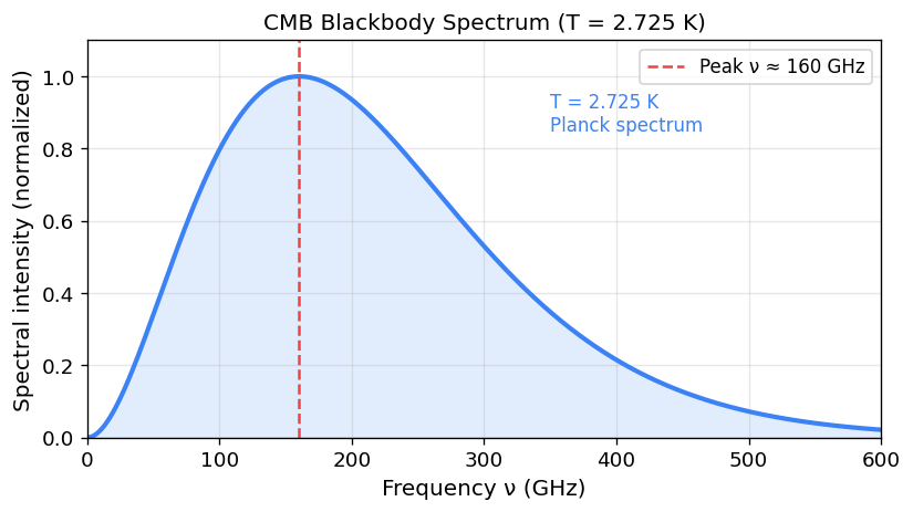
The cosmic microwave background is a near-perfect blackbody at temperature:

\[T_0 = 2.725 \text{ K}.\]

Its energy density is \(\varepsilon_{\gamma,0} = \alpha T_0^4 = 0.2606 \text{ MeV m}^{-3}\) (where \(\alpha = 4\sigma/c\) is the radiation constant), giving a density parameter:

\[\Omega_{\gamma,0} = \frac{\varepsilon_{\gamma,0}}{\varepsilon_{c,0}} \approx 5 \times 10^{-5}.\]

Despite its tiny contribution to the current energy budget, the CMB photons outnumber baryons enormously. The photon number density is:

\[n_{\gamma,0} = 0.2436\left(\frac{kT_0}{\hbar c}\right)^3 \approx 410 \text{ cm}^{-3} = 4.107 \times 10^8 \text{ m}^{-3},\]

while the baryon number density is \(n_{b,0} \approx 0.25 \text{ m}^{-3}\). The baryon-to-photon ratio:

\[\eta = \frac{n_b}{n_\gamma} \approx 6.1 \times 10^{-10},\]

is conserved throughout cosmic history (after \(e^+e^-\) annihilation). For every baryon in the universe, there are roughly 1.6 billion CMB photons.

Photon–Matter Coupling and Thomson Scattering

Before recombination, the universe was a hot plasma of protons, electrons, and photons. Photons scattered off free electrons via Thomson scattering with cross-section \(\sigma_T = 6.65 \times 10^{-29} \text{ m}^2\). The scattering rate was:

\[\Gamma = n_e \sigma_T c = \frac{n_{b,0}}{a^3}\sigma_T c,\]

which was much greater than the Hubble rate \(H\) at early times. While \(\Gamma \gg H\), photons and baryons were tightly coupled, forming a photon-baryon fluid. This coupling is responsible for the acoustic oscillations imprinted on both the CMB power spectrum and the matter power spectrum.

Recombination and Decoupling

As the universe cooled, free electrons combined with protons to form neutral hydrogen — the epoch of recombination. The fractional ionization \(X = n_p/(n_p + n_H)\) is governed by the Saha equation:

\[\frac{1-X}{X^2} = 3.84\eta \left(\frac{kT}{m_e c^2}\right)^{3/2} \exp\!\left(\frac{Q}{kT}\right),\]

where \(Q = 13.6 \text{ eV}\) is the ionization energy of hydrogen. The rapid exponential dependence on \(T\) means recombination happens quickly: the fractional ionization drops from \(X = 0.9\) at \(z = 1480\) to \(X = 0.1\) at \(z = 1260\). The recombination temperature is:

\[kT_{\text{rec}} = \frac{Q}{42} \approx 0.324 \text{ eV}, \quad T_{\text{rec}} \approx 3760 \text{ K}, \quad z_{\text{rec}} \approx 1380.\]

(A more careful calculation accounting for the photon statistics gives \(z_{\text{dec}} \approx 1100\), the standard redshift of last scattering.) The recombination temperature is much lower than the naive estimate \(T \sim Q/k \approx 60{,}000 \text{ K}\), because the vast photon-to-baryon ratio means the high-energy tail of the blackbody spectrum can keep hydrogen ionized even when the mean photon energy is far below the ionization threshold.

Once the free electron density plummeted, photons could no longer scatter efficiently — the universe became transparent. The surface of last scattering at \(z_{\text{dec}} \approx 1100\) is the origin of all CMB photons we receive today. Surrounding every observer in the universe is a spherical shell, some 46 Gpc away in co-moving coordinates, from which these photons have been streaming freely for 13.4 billion years.

CMB Anisotropies and the Angular Power Spectrum

The CMB is remarkably uniform, but the Planck and WMAP satellites revealed small temperature fluctuations:

\[\frac{\delta T}{T}(\theta,\phi) \equiv \frac{T(\theta,\phi) - \langle T\rangle}{\langle T\rangle}, \quad \left\langle\left(\frac{\delta T}{T}\right)^2\right\rangle^{1/2} \approx 1.1 \times 10^{-5}.\]

These anisotropies are the imprints of primordial density fluctuations, stretched and amplified by the acoustic oscillations of the photon-baryon fluid before decoupling. The fluctuation field is expanded in spherical harmonics:

\[\frac{\delta T}{T}(\theta,\phi) = \sum_{\ell=0}^\infty \sum_{m=-\ell}^{\ell} a_{\ell m} Y_\ell^m(\theta,\phi),\]

and the angular power spectrum \(C_\ell = \langle |a_{\ell m}|^2 \rangle\) captures the amplitude of fluctuations on angular scale \(\theta \approx \pi/\ell\). A plot of \(\ell(\ell+1)C_\ell/2\pi\) against \(\ell\) reveals a series of acoustic peaks:

• First acoustic peak at \(\ell \approx 200\) (\(\theta \approx 1°\)): the sound horizon at decoupling, projected onto the sky. Its angular position constrains the total density parameter \(\Omega_{\text{total}} \approx 1\) — the universe is flat.
• Second acoustic peak at \(\ell \approx 540\): the ratio of odd to even peak heights constrains the baryon density \(\Omega_b h^2\).
• Higher peaks: their positions and heights constrain \(H_0\), the dark matter density, and the primordial spectrum of fluctuations.

The combination of CMB temperature and polarization data from Planck provides a powerful, multi-dimensional probe of cosmological parameters, yielding the precision constraints discussed in Chapter 13.

---

Section 3.2: Structure Formation

The Galaxy Correlation Function

The large-scale distribution of galaxies is not perfectly uniform — it mirrors (in a biased way) the underlying dark matter density field. The two-point correlation function \(\xi(r)\) quantifies the excess probability of finding two galaxies separated by distance \(r\), compared to a random distribution:

\[\xi(r) = \left\langle \delta(\mathbf{x})\, \delta(\mathbf{x}+\mathbf{r})\right\rangle,\]

where \(\delta(\mathbf{x}) = (\rho(\mathbf{x}) - \bar\rho)/\bar\rho\) is the fractional overdensity. Observations of galaxy surveys give a power-law fit on scales \(r \lesssim 10 \text{ Mpc}\):

\[\xi(r) \approx \left(\frac{r}{r_0}\right)^{-\gamma},\]

with correlation length \(r_0 \approx 5 \text{ Mpc}\) and slope \(\gamma \approx 1.8\). This means galaxies cluster strongly on small scales and are nearly uncorrelated on scales much larger than \(r_0\).

Linear Growth of Structure

In the linear regime (small \(\delta\)), perturbations in the dark matter density grow by gravitational instability. During matter domination, a density perturbation on scales well below the Hubble radius grows as:

\[\delta \propto a(t) \propto t^{2/3}.\]

This is the linear growth law. In the radiation-dominated era, growth is suppressed (the Meszaros effect) because the rapid expansion prevents perturbations from collapsing. Structure therefore begins to grow efficiently only after matter-radiation equality at \(z_{eq} \approx 3400\).

On scales above the Jeans length, the primordial fluctuation spectrum (approximately scale-invariant, \(P(k) \propto k^{n_s}\) with \(n_s \approx 0.96\)) is processed into the observed matter power spectrum \(P(k)\) by the transfer function, which encodes the suppression of small-scale modes during radiation domination.

Galaxy Bias

Galaxies do not trace the dark matter distribution perfectly. The bias parameter \(b\) relates the galaxy overdensity to the matter overdensity:

\[\delta_{\text{gal}} = b \, \delta_{\text{dm}}.\]

Massive, elliptical galaxies in dense environments tend to have \(b > 1\) (they are over-represented in high-density regions), while dwarf galaxies have \(b \lesssim 1\). Understanding the bias is essential for extracting the underlying cosmological signal from galaxy surveys.

---

Section 3.3: The Early Universe — Thermal History and Baryogenesis

Time–Temperature Correspondence

In the radiation-dominated era, the energy density is \(\rho_r c^2 = g_* (\pi^2/30)(kT)^4/(\hbar c)^3\), where \(g_*\) is the number of relativistic degrees of freedom. The Friedmann equation then gives the fundamental time–temperature relation:

\[t \approx \left(\frac{45 \hbar^3 c^5}{16\pi^3 G g_*}\right)^{1/2} \frac{1}{(kT)^2} \approx \frac{2.4}{\sqrt{g_*}} \left(\frac{\text{MeV}}{kT}\right)^2 \text{ s}.\]

Some landmark values:

• \(kT \sim 1 \text{ GeV}\): \(t \sim 10^{-6} \text{ s}\) (QCD phase transition)
• \(kT \sim 1 \text{ MeV}\): \(t \sim 1 \text{ s}\) (neutrino decoupling, start of BBN)
• \(kT \sim 1 \text{ keV}\): \(t \sim 10^6 \text{ s}\) (\(\sim 10 \text{ days}\))

Neutrino Decoupling and \(e^+e^-\) Annihilation

At \(kT \sim 3\) MeV, the rate of weak interactions maintaining neutrino equilibrium falls below the Hubble rate, and neutrinos decouple from the photon-electron plasma. Shortly after, at \(kT \sim m_e c^2 = 0.511 \text{ MeV}\), the electron-positron pairs annihilate, dumping entropy into the photon gas but not the already-decoupled neutrinos. By entropy conservation, this heats the photons by a factor \((11/4)^{1/3}\), while the neutrino temperature remains unchanged. The neutrino temperature today is therefore:

\[T_\nu = \left(\frac{4}{11}\right)^{1/3} T_\gamma \approx 0.714 \times 2.725 \text{ K} = 1.945 \text{ K}.\]

This prediction is confirmed indirectly through its effects on BBN and the CMB, and the effective number of neutrino species \(N_{\text{eff}} \approx 3.1\) measured from Planck data is consistent with three Standard Model neutrino flavors.

Matter–Radiation Equality

The universe transitions from radiation domination to matter domination when \(\rho_m = \rho_r\), i.e., when:

\[\Omega_{m,0}\,(1+z_{eq})^3 = \Omega_{r,0}\,(1+z_{eq})^4 \implies 1+z_{eq} = \frac{\Omega_{m,0}}{\Omega_{r,0}} \approx 3400.\]

This transition is crucial for structure formation: during radiation domination, the rapid expansion suppresses gravitational collapse (Meszaros effect), so structure can only grow efficiently after \(z_{eq}\).

Baryogenesis and the Sakharov Conditions

The observed universe contains baryons but essentially no antibaryons — a baryon asymmetry of \(\eta = n_b/n_\gamma \approx 6 \times 10^{-10}\). Yet physics as we understand it is almost perfectly symmetric under charge conjugation and parity (CP). How did the asymmetry arise? Andrei Sakharov (1967) identified three necessary conditions for dynamically generating a baryon asymmetry:

1. Baryon number violation: Processes must exist that can create or destroy net baryons.
2. C and CP violation: The laws of physics must distinguish matter from antimatter, so baryon-creating reactions proceed at different rates than baryon-destroying reactions.
3. Departure from thermal equilibrium: In thermal equilibrium, detailed balance ensures that net baryon production vanishes even in the presence of B and CP violation.

The Standard Model satisfies all three conditions in principle, but the degree of CP violation in the quark sector and the nature of the electroweak phase transition appear insufficient to explain the observed \(\eta\). The origin of baryogenesis remains an open problem, with candidates ranging from leptogenesis (via heavy Majorana neutrino decays) to electroweak baryogenesis (via first-order phase transitions in extensions of the Standard Model).

---

Section 3.4: Big Bang Nucleosynthesis

Historical Background

Big Bang Nucleosynthesis (BBN) was the first theoretical success of the Hot Big Bang model. In 1948, Ralph Alpher, Hans Bethe, and George Gamow published the famous “αβγ paper” predicting that the light elements were forged in the first few minutes of cosmic history. (Bethe’s name was added by Gamow for alphabetical aesthetics — Bethe had no involvement in the calculation.) The prediction of the cosmic helium abundance \(Y_4 \approx 0.25\) — confirmed by stellar observations — is one of the pillars of modern cosmology.

The n/p Ratio

At temperatures above \(kT \sim\) a few MeV, weak interactions maintain thermal equilibrium between neutrons and protons:

\[n + \nu_e \rightleftharpoons p + e^-, \quad n + e^+ \rightleftharpoons p + \bar\nu_e.\]

In thermal equilibrium at temperature \(T\), the neutron-to-proton ratio is:

\[\frac{n}{p} = \exp\!\left(-\frac{\Delta m c^2}{kT}\right),\]

where \(\Delta m c^2 = (m_n - m_p)c^2 = 1.293 \text{ MeV}\). As the universe cools, this ratio decreases. At \(kT \sim 1\) MeV, the weak reaction rate drops below the Hubble rate — the n/p ratio freezes out at approximately:

\[\left.\frac{n}{p}\right|_{\text{freeze}} \approx \frac{1}{5}.\]

After freeze-out, neutrons continue to decay via \(n \to p + e^- + \bar\nu_e\) with mean lifetime \(\tau_n \approx 880 \text{ s}\). By the time nucleosynthesis begins at \(kT \sim 0.1 \text{ MeV}\) (\(t \sim 200 \text{ s}\)), neutron decay has reduced the ratio to:

\[\frac{n}{p} \approx \frac{1}{7}.\]

Light Element Synthesis

Below \(kT \sim 0.1\) MeV, the universe cools enough that deuterium can survive photodisintegration (the deuterium bottleneck). Once deuterium survives, a rapid chain of reactions synthesizes helium-4:

\[p + n \to D + \gamma, \quad D + D \to {}^3\text{He} + n, \quad {}^3\text{He} + D \to {}^4\text{He} + p.\]

Virtually all available neutrons end up in helium-4 nuclei. With \(n/p = 1/7\), the mass fraction of helium-4 is:

\[Y_4 = \frac{4 \times (n/2)}{n + p} = \frac{2n/p}{1 + n/p} = \frac{2/7}{1 + 1/7} = \frac{2}{8} = 0.25.\]

A slightly more careful calculation accounting for neutron decay during nucleosynthesis gives \(Y_4 \approx 0.24\), in excellent agreement with the observed primordial helium abundance.

Primordial Abundances

The remaining nucleons produce trace amounts of other light elements:

Element	Primordial Mass Fraction	Notes
\({}^1\text{H}\)	\(\sim 0.75\)	Dominant
\({}^4\text{He}\)	\(\sim 0.24\)	\(Y_4\) sensitive to \(n/p\) ratio
\({}^2\text{D}\) (Deuterium)	\(\sim 2 \times 10^{-5}\)	Sensitive probe of \(\Omega_b\)
\({}^7\text{Li}\)	\(\sim 5 \times 10^{-10}\)	Observed lithium problem

The deuterium abundance is exquisitely sensitive to the baryon density: higher \(\Omega_b\) → more efficient D-burning → lower D/H. Measurements of primordial deuterium in pristine quasar absorption systems give \(\Omega_b h^2 = 0.022 \pm 0.002\), consistent with the CMB-derived value. The slight discrepancy in the lithium-7 abundance (\(\sim 3\times\) lower than predicted) is the lithium problem and remains unresolved.

BBN provides an independent measurement of the baryon density \(\Omega_b \approx 0.048 \pm 0.003\), in agreement with CMB observations. This concordance is one of the great successes of the Big Bang model.

---

Section 3.5: Inflation

Problems with the Standard Big Bang

The Hot Big Bang model, despite its many successes, has three serious fine-tuning problems when extrapolated back to very early times.

The Flatness Problem. The Friedmann equation can be written as:

\[\Omega(a) - 1 = \frac{kc^2}{a^2 H^2}.\]

During radiation or matter domination, \(aH = \dot{a}\) decreases with time, so \(|\Omega - 1| = kc^2/(aH)^2\) grows. The observed flatness \(|\Omega_0 - 1| \lesssim 0.01\) requires exquisite fine-tuning of the initial conditions. At the Planck time (\(t \sim 10^{-43}\) s), the universe must have satisfied \(|\Omega - 1| \lesssim 10^{-60}\) — a staggering coincidence demanding explanation.

The Horizon Problem. The CMB is isotropic to one part in \(10^5\) across the entire sky. Yet in the standard Big Bang, the particle horizon at recombination subtends only about 1° on the sky. Regions of the CMB separated by more than 1° were causally disconnected at decoupling — they could never have exchanged information or reached thermal equilibrium. How, then, is the sky so uniform on 10° or 100° scales?

The Monopole Problem. Grand Unified Theories (GUTs) predict that magnetic monopoles — topological defects — should be produced copiously during the GUT phase transition at \(kT \sim 10^{16}\) GeV (\(t \sim 10^{-36}\) s). Each monopole weighs \(\sim 10^{16}\) GeV. Standard cosmology predicts a monopole density comparable to the baryon density — yet no monopole has ever been detected.

The Inflationary Solution

Inflation, proposed by Alan Guth (1981) and developed by Andrei Linde, Alexei Starobinsky, and others, resolves all three problems with a single mechanism: a brief period of exponential expansion in the very early universe, driven by a scalar field (the inflaton) with nearly constant potential energy.

During inflation, the energy density is dominated by the potential energy \(V(\phi)\) of the inflaton, acting like a cosmological constant with equation of state \(w \approx -1\). The scale factor grows exponentially:

\[a \propto e^{H_{\text{inf}}t}, \quad H_{\text{inf}} = \sqrt{\frac{8\pi G V}{3c^2}} \approx \text{const}.\]

This requires the null energy condition to be violated: \(\rho + P/c^2 < 0\), i.e., \(P < -\rho c^2\) and \(w < -1/3\). The inflaton in slow-roll inflation satisfies this automatically when the potential is nearly flat.

The quantitative requirement for solving the horizon problem is that inflation produces at least:

\[N = \ln\frac{a_f}{a_i} \geq 54 \text{ e-folds}.\]

This is the number of factors of \(e\) by which the universe expanded during inflation. During 54 e-folds, the inflationary patch grows by a factor of \(e^{54} \approx 4 \times 10^{23}\), so a region that was initially causally connected — small enough to thermalize — expands to encompass our entire observable universe today.

Resolution of the problems:

• Flatness: During inflation, \(aH = a\dot H + \dot a H = \dot a H\) grows exponentially (\(\dot a = aH = \text{const} \times a\)), so \(|\Omega - 1| = kc^2/(aH)^2 \to 0\) — any initial curvature is inflated away.
• Horizon: The observable universe descended from a region small enough to have been in causal contact before inflation.
• Monopoles: Diluted to negligible density by the exponential expansion.

Reheating and Quantum Fluctuations

Inflation ends when the inflaton rolls to the minimum of its potential and oscillates, decaying into Standard Model particles — a process called reheating. The universe thermalizes and enters the radiation-dominated phase of the standard Big Bang.

But inflation does more than solve fine-tuning problems: it provides the seeds of all cosmic structure. Quantum fluctuations in the inflaton field — inevitable due to the Heisenberg uncertainty principle — are stretched to macroscopic scales by the exponential expansion. These primordial perturbations have an approximately scale-invariant (Harrison–Zel’dovich) power spectrum:

\[P(k) \propto k^{n_s}, \quad n_s \approx 0.96,\]

where \(n_s = 1\) is exactly scale-invariant. The slight red tilt (\(n_s < 1\)) reflects the slow roll of the inflaton. These perturbations seed the CMB anisotropies and the large-scale structure of the universe — two completely different observables that are both explained by the same inflationary mechanism, providing powerful evidence for inflation.

Inflation also predicts a background of primordial gravitational waves (tensor perturbations), characterized by the tensor-to-scalar ratio \(r\). Detection of the B-mode polarization signal in the CMB from these gravitational waves would be a smoking gun for inflation.

---

Chapter 4: The Big Bang, Black Holes, and the Far Future

Section 4.1: Singularities, Quantum Gravity, and the Origin of Time

Penrose Diagrams

Penrose diagrams (conformal diagrams) provide a powerful way to visualize the causal structure of spacetimes. By rescaling time and spatial coordinates with conformal transformations that bring infinity to a finite distance on the diagram, Penrose diagrams compress infinite spacetimes into finite pictures while preserving the 45° light-cone structure.

In a Penrose diagram, the FRW universe has a beginning — the Big Bang singularity — as a spacelike surface at the bottom. Null rays at 45° show that our past light cone originates from a finite region of the Big Bang, explaining the horizon problem. During inflation, light cones can reach across the entire observable universe, resolving the horizon problem diagrammatically.

The Classical Singularity

The Big Bang singularity — the initial state of infinite density and curvature at \(t = 0\) — is a formal breakdown of classical general relativity, analogous to the ultraviolet catastrophe in blackbody radiation or the singularity of the hydrogen atom in classical electrodynamics. Just as quantum mechanics resolved the hydrogen singularity (the ground state has finite, nonzero radius), quantum gravity is expected to resolve the Big Bang singularity.

The Planck mass sets the scale at which quantum gravitational effects become important:

\[M_P c^2 = \sqrt{\frac{\hbar c^5}{G}} \approx 10^{19} \text{ GeV} \approx 2.2 \times 10^{-8} \text{ kg}.\]

The corresponding Planck length is \(\ell_P = \hbar/(M_P c) \approx 1.6 \times 10^{-35} \text{ m}\) and Planck time \(t_P \approx 5.4 \times 10^{-44} \text{ s}\). For \(t < t_P\), a quantum theory of gravity is required, and classical GR cannot be trusted.

Approaches to Quantum Gravity

Several approaches attempt to quantize gravity:

• String Theory: Models elementary particles as one-dimensional vibrating strings. Gravity emerges naturally as a massless spin-2 excitation (the graviton). Requires extra spatial dimensions (typically 6 or 7) compactified at the Planck scale. Provides a consistent perturbative theory of quantum gravity but has not yet made definitive testable predictions.
• Loop Quantum Gravity (LQG): Quantizes the gravitational field directly, leading to a discrete structure of spacetime at the Planck scale. Space is composed of discrete “atoms” with minimum area \(\sim \ell_P^2\) and volume \(\sim \ell_P^3\).
• Causal Dynamical Triangulation: Constructs spacetime as a simplicial complex and sums over geometries (a discrete path integral for gravity).
• Emergent Gravity: Gravity is not fundamental but emerges from the entanglement structure of an underlying quantum many-body system (Verlinde’s entropic gravity, et al.).

The Big Bounce

In LQG, the Big Bang singularity is replaced by a Big Bounce: the universe contracted from a previous phase, quantum effects generated a repulsive force at Planck density, and the universe bounced into the expanding phase we observe. This is sometimes called Loop Quantum Cosmology. In this picture, the universe is eternal — it oscillates or extends infinitely into the past, eliminating the need for a creation event. The predictions of LQC for the CMB spectrum are under active investigation.

---

Chapter 5: Neutrino Cosmology, Precision Measurements, and Dark Matter Halos

Section 5.1: Neutrino Cosmology

Beta Decay and the Neutrino

The neutrino was proposed by Wolfgang Pauli in 1930 to explain the continuous energy spectrum of electrons in nuclear beta decay:

\[n \to p + e^- + \bar\nu_e.\]

The weak interaction responsible for beta decay is mediated by the \(W^\pm\) and \(Z^0\) bosons, with Fermi coupling constant \(G_F/(\hbar c)^3 \approx 1.17 \times 10^{-5} \text{ GeV}^{-2}\). The Standard Model contains three neutrino flavors: electron neutrino \(\nu_e\), muon neutrino \(\nu_\mu\), and tau neutrino \(\nu_\tau\), along with their antiparticles — six neutrino species in total.

Relic Neutrino Background

Analogous to the CMB photons, there exists a cosmic neutrino background (CνB) — a thermal relic from the epoch when the universe was dense enough to maintain neutrinos in equilibrium. After neutrino decoupling and \(e^+e^-\) annihilation, the neutrino temperature is \(T_\nu = (4/11)^{1/3} T_\gamma\). The number density of each neutrino flavor (plus antineutrinos) is:

\[n_\nu = \frac{3}{4} \times \frac{2}{2} \times \frac{4}{11} \times n_\gamma \implies n_{\nu,\text{total}} = 3 \times \frac{3}{11} n_\gamma = \frac{9}{11}(4.107 \times 10^8 \text{ m}^{-3}) = 3.36 \times 10^8 \text{ m}^{-3}.\]

At any moment, roughly twenty million cosmic neutrinos per species are streaming through every cubic centimeter of space — and through your body.

Neutrino Masses and the Effective Number of Species

Neutrino oscillation experiments — which observe transitions between neutrino flavors — establish that at least two of the three neutrinos have nonzero mass. The mass squared splittings are:

\[\Delta m_{21}^2 \approx 7.5 \times 10^{-5} \text{ eV}^2, \quad |\Delta m_{31}^2| \approx 2.5 \times 10^{-3} \text{ eV}^2.\]

These give a lower bound on the heaviest neutrino mass \(m_3 \gtrsim 0.05 \text{ eV}\), but do not constrain absolute masses. Cosmological observations (CMB + large-scale structure) provide upper bounds: \(\sum m_\nu < 0.2 \text{ eV}\), corresponding to \(\Omega_\nu < 0.007\).

If neutrinos provided all the nonbaryonic dark matter, they would need \(m_\nu c^2 \approx 3.8 \text{ eV}\) — ruled out by the above bound. Moreover, neutrinos are hot dark matter (relativistic at decoupling), which would wash out small-scale structure inconsistent with the observed galaxy distribution. The dark matter must be cold (non-relativistic at decoupling), ruling out Standard Model neutrinos as the primary dark matter component.

The effective number of neutrino species is measured from the CMB through its effect on the radiation density at decoupling: \(N_{\text{eff}} = 3.1 \pm 0.4\), consistent with three Standard Model flavors.

---

Section 5.2: Precision Cosmology and the \(\Lambda\)CDM Standard Model

The Six-Parameter Model

Modern cosmological observations are fit by the \(\Lambda\)CDM model — cold dark matter plus a cosmological constant — characterized by six fundamental parameters. The Planck 2015 satellite data yield:

Parameter	Value	Physical Meaning
\(h\)	\(\approx 0.673\)	\(H_0 = 100h \text{ km s}^{-1}\text{Mpc}^{-1}\)
\(\Omega_{dm}h^2\)	\(\approx 0.119\)	Physical cold dark matter density
\(\Omega_b h^2\)	\(\approx 0.022\)	Physical baryon density
\(n_s\)	\(\approx 0.960\)	Scalar spectral index
\(\Delta^2_0\)	\(\approx 2.2 \times 10^{-9}\)	Amplitude of primordial fluctuations
\(\tau\)	\(\approx 0.066\)	Optical depth to reionization

From these six numbers, all other cosmological quantities are derived:

• \(\Omega_m = \Omega_{dm} + \Omega_b \approx 0.31\)
• \(\Omega_\Lambda \approx 0.69\) (from flatness: \(\Omega_m + \Omega_\Lambda = 1\))
• \(t_0 \approx 13.8 \text{ Gyr}\)
• \(z_{\text{dec}} \approx 1100\), \(z_{eq} \approx 3400\)

Auxiliary Parameters

Beyond the vanilla \(\Lambda\)CDM, several additional parameters may be needed:

• Equation of state \(w\): If dark energy is not a cosmological constant (\(w = -1\)), but a dynamical scalar field, \(w \neq -1\). Current data are consistent with \(w = -1\) to about 5%.
• Running of the spectral index \(n_r = dn_s/d\ln k\): Deviations from exact power-law inflation.
• Tensor-to-scalar ratio \(r\): Amplitude of primordial gravitational waves. Currently \(r < 0.1\).
• Sum of neutrino masses \(\sum m_\nu\): Currently constrained to \(<0.2 \text{ eV}\).
• Effective number of relativistic species \(N_{\text{eff}}\): Deviations from 3.046 would indicate new light particles.

Bayesian Parameter Estimation

Cosmological parameter inference is done within the Bayesian framework. The posterior probability of a parameter set \(\boldsymbol{\theta}\) given data \(D\) is:

\[P(\boldsymbol{\theta} | D) \propto \mathcal{L}(D | \boldsymbol{\theta}) \times \pi(\boldsymbol{\theta}),\]

where \(\mathcal{L}\) is the likelihood and \(\pi(\boldsymbol{\theta})\) is the prior. For Gaussian errors, the likelihood is related to the chi-squared statistic:

\[\chi^2 = \sum_i \frac{(O_i - T_i(\boldsymbol{\theta}))^2}{\sigma_i^2}, \quad \mathcal{L} \propto e^{-\chi^2/2}.\]

The posterior is explored using Markov Chain Monte Carlo (MCMC) algorithms, which sample the high-dimensional parameter space efficiently. The resulting posterior distributions for each parameter give confidence intervals that marginalize over all other parameters.

---

Section 5.3: Dark Matter Halos — Spherical Collapse and the Mass Function

The Spherical Collapse Model

The formation of dark matter halos from primordial overdensities is captured by the spherical collapse model. Consider a spherical region of matter with a slight overdensity \(\delta_i > 0\) at some early time. Gravity decelerates this region relative to the background Hubble flow; if the overdensity is large enough, the sphere eventually detaches from the expansion and collapses.

The exact evolution of a spherical overdensity can be parametrized in terms of a development angle \(\theta\) (for a closed effective geometry):

\[a(\theta) = A(1 - \cos\theta), \quad t(\theta) = B(\theta - \sin\theta),\]

where \(A\) and \(B\) are constants determined by the overdensity amplitude. The collapse singularity (\(\theta = 2\pi\)) occurs at \(t_{\text{coll}} = 2\pi B\). By the time of collapse, the linear overdensity (extrapolated from the linear growth law) has reached the linear collapse threshold:

\[\delta_c = \frac{3}{20}(12\pi)^{2/3} \approx 1.686.\]

In practice, real halos do not collapse to a singularity but virialize at roughly half the turnaround radius, reaching a density contrast of \(\Delta_c \approx 178\) relative to the background. The virial radius \(r_{\text{vir}}\) is defined as the radius within which the mean density is \(200\) times the critical density.

The NFW Profile

Cosmological N-body simulations reveal a universal density profile for dark matter halos, proposed by Navarro, Frenk, and White (1997):

\[\rho_{\text{NFW}}(r) = \frac{\rho_s}{\left(\frac{r}{r_s}\right)\left(1 + \frac{r}{r_s}\right)^2},\]

where \(\rho_s\) is the characteristic density and \(r_s\) is the scale radius. The NFW profile has two key features: \(\rho \propto r^{-1}\) at small radii (cuspy center) and \(\rho \propto r^{-3}\) at large radii. The concentration parameter \(c_{\text{vir}} = r_{\text{vir}}/r_s\) characterizes how centrally concentrated the halo is; massive halos typically have \(c_{\text{vir}} \sim 4\)–\(6\), while less massive halos can have \(c_{\text{vir}} \sim 10\)–\(20\).

The cumulative mass within radius \(r\) for the NFW profile is:

\[M(r) = 4\pi \rho_s r_s^3 \left[\ln\!\left(1 + \frac{r}{r_s}\right) - \frac{r/r_s}{1 + r/r_s}\right],\]

and the circular velocity \(v_c(R) = \sqrt{GM(R)/R}\) rises from zero at the center, peaks near \(r \approx 2r_s\), and declines at large radii — producing a rotation curve consistent with observations when embedded in a disk galaxy.

The Press-Schechter Mass Function

How many dark matter halos of a given mass exist per unit volume? The Press-Schechter formalism (1974) answers this by treating halo formation as a threshold-crossing problem for a Gaussian density field. The number density of halos in the mass range \([M, M + dM]\) is:

\[\frac{dn}{dM} = \sqrt{\frac{2}{\pi}} \frac{\bar\rho}{M^2} \frac{\delta_c}{\sigma(M)} \left|\frac{d\ln\sigma}{d\ln M}\right| \exp\!\left(-\frac{\delta_c^2}{2\sigma^2(M)}\right),\]

where \(\sigma^2(M)\) is the variance of the density field smoothed on the mass scale \(M\), and \(\bar\rho\) is the mean matter density. The exponential factor suppresses the abundance of halos with \(M \gg M_*(z)\), where \(M_*\) is the characteristic nonlinear mass scale at redshift \(z\) defined by \(\sigma(M_*) = \delta_c\).

The Press-Schechter function predicts a steep decline in the abundance of massive clusters and a power-law increase in the number of low-mass halos. Observed cluster mass functions at various redshifts provide powerful constraints on \(\sigma_8\) (the amplitude of the power spectrum on 8 Mpc scales) and \(\Omega_m\).

---

Appendices

Appendix A: High-Frequency Photon Number Density

The number density of photons with frequency greater than \(\nu_0\) in a blackbody distribution is found by integrating the Planck distribution in the high-frequency (Wien) tail:

\[n(\nu > \nu_0) = \frac{8\pi}{c^3}\int_{\nu_0}^\infty \frac{\nu^2 d\nu}{\exp(h\nu/kT) - 1} \approx \frac{8\pi}{c^3}\int_{\nu_0}^\infty \nu^2 e^{-h\nu/kT} d\nu.\]

In the Wien approximation (\(h\nu_0 \gg kT\)), this gives:

\[n(\nu > \nu_0) \approx \frac{8\pi}{c^3}\left(\frac{kT}{h}\right)^3 e^{-h\nu_0/kT}\left[\left(\frac{h\nu_0}{kT}\right)^2 + 2\frac{h\nu_0}{kT} + 2\right].\]

This expression is useful for computing the rate of photoionization reactions, where only photons with energy above the ionization threshold \(h\nu_0 = Q\) contribute.

Appendix B: Scale Factor Solutions by Dominant Era

The following table summarizes the evolution of the scale factor, density, and Hubble parameter in each single-component dominated era:

Era	\(w\)	\(\rho(a)\)	\(a(t)\)	\(\rho(t)\)
Radiation	\(1/3\)	\(\propto a^{-4}\)	\(\propto t^{1/2}\)	\(\propto t^{-2}\)
Matter	\(0\)	\(\propto a^{-3}\)	\(\propto t^{2/3}\)	\(\propto t^{-2}\)
Curvature	\(-1/3\)	\(\propto a^{-2}\)	\(\propto t\)	\(\propto t^{-2}\)
Dark Energy (\(\Lambda\))	\(-1\)	\(= \text{const}\)	\(\propto e^{Ht}\)	\(= \text{const}\)

Note that in every era, \(\rho \propto t^{-2}\) — a remarkable coincidence that follows directly from the Friedmann equation when only one component dominates.

Appendix C: Age of the Universe

The age of the universe is:

\[t_0 = \frac{1}{H_0}\int_0^1 \frac{da}{a \, E(a)},\]

where the dimensionless Hubble function is:

\[E(a) = \frac{H(a)}{H_0} = \sqrt{\Omega_{r,0}\,a^{-4} + \Omega_{m,0}\,a^{-3} + \Omega_{k,0}\,a^{-2} + \Omega_{\Lambda,0}}.\]

For the Benchmark Model (\(\Omega_m = 0.31\), \(\Omega_\Lambda = 0.69\), \(\Omega_r \approx 0\), \(k = 0\)):

\[t_0 = \frac{1}{H_0}\int_0^1 \frac{da}{\sqrt{0.31 a^{-1} + 0.69 a^2}} \approx \frac{0.964}{H_0} \approx 13.8 \text{ Gyr}.\]

Appendix D: The Big Crunch and Closed Universe Dynamics

For a closed universe (\(k = +1\)) with matter and no cosmological constant, the Friedmann equation has the parametric solution:

\[a(\theta) = \frac{\Omega_{m,0}}{2(\Omega_{m,0} - 1)}(1 - \cos\theta), \quad t(\theta) = \frac{\Omega_{m,0}}{2H_0(\Omega_{m,0}-1)^{3/2}}(\theta - \sin\theta).\]

The universe reaches maximum expansion at \(\theta = \pi\):

\[a_{\max} = \frac{\Omega_{m,0}}{\Omega_{m,0} - 1}, \quad t_{\max} = \frac{\pi\,\Omega_{m,0}}{2H_0(\Omega_{m,0}-1)^{3/2}},\]

and recollapses to a Big Crunch singularity at \(\theta = 2\pi\), exactly twice the time to maximum expansion: \(t_{\text{crunch}} = 2t_{\max}\). The Big Crunch is in every way the time-reverse of the Big Bang. With a cosmological constant \(\Lambda > 0\), a closed universe can avoid recollapse if \(\Omega_\Lambda\) is large enough — consistent with what we observe.