Chapter 1: Introduction and Linear Second Order ODEs

What is an Ordinary Differential Equation?

A good portion of this course is devoted to the study of linear, second-order ordinary differential equations (ODEs). You have already seen a special case of these in AMATH 250 or 251, namely, linear, second-order DEs with constant coefficients. With these ODEs, one is already able to model a number of interesting natural phenomena. But linear, second order ODEs arise in a wide variety of applications in both classical and quantum mechanics.

For example, \( y'' + 25y = 0 \) is a linear second-order ODE, while \( y'' + \sin y = 0 \) is nonlinear.

The Standard Form of a Linear Second-Order ODE

The most general linear second-order ODE in \( y(x) \) is

\[ a_2(x)y'' + a_1(x)y' + a_0(x)y = f(x), \qquad x \in I. \]

Assuming \( a_2(x) \) is not identically zero, we divide through to obtain the standard or normalized form:

\[ y'' + P(x)y' + Q(x)y = R(x), \]

where \( P(x) = a_1/a_2 \), \( Q(x) = a_0/a_2 \), and \( R(x) = f/a_2 \). The homogeneous DE associated with this is

\[ y'' + P(x)y' + Q(x)y = 0. \]

When \( R(x) = 0 \), the DE is said to be homogeneous. The solution structure for the inhomogeneous case builds directly on that of the homogeneous case, as we shall soon see.

General Solutions and Initial Value Problems

In your previous course, you learned that the general solution of a second-order homogeneous constant-coefficient DE involves two arbitrary constants. The same is true for the general case: the solution space of a second-order linear homogeneous ODE is two-dimensional. We will prove this rigorously in Chapter 7.

To extract a unique solution from this two-parameter family, one imposes initial conditions at some point \( x_0 \in I \):

\[ y(x_0) = A, \qquad y'(x_0) = B, \]

where \( A, B \in \mathbb{R} \). Geometrically, this selects the unique solution curve passing through the point \( (x_0, A) \) with tangent slope \( B \) there.

Special Functions: A Preview

Many important second-order ODEs with nonconstant coefficients arise in applications, and their solutions are given special names. We list the most important families here as motivation for later chapters.

Bessel’s equation (arising from Laplace’s equation in polar coordinates, e.g., vibration of a circular membrane):

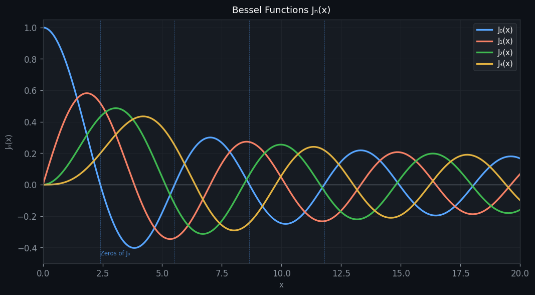
\[ x^2 y'' + xy' + (x^2 - p^2)y = 0. \]

For \( p = 0, 1, 2, \ldots \), the regular solutions are the Bessel functions \( J_0(x), J_1(x), J_2(x), \ldots \), which are oscillatory with infinitely many zeros.

Legendre’s equation (arising from the angular part of Laplace’s equation in spherical coordinates):

\[ (1 - x^2)y'' - 2xy' + p(p+1)y = 0. \]

For \( p = n = 0, 1, 2, \ldots \), the polynomial solutions are the Legendre polynomials \( P_n(x) \).

Laguerre’s equation (related to the radial part of the hydrogen atom quantum eigenfunctions):

\[ xy'' + (1-x)y' + ay = 0. \]

Hermite’s equation (eigenfunctions of the quantum harmonic oscillator):

\[ y'' - 2xy' + 2ay = 0. \]

These ODEs all have singular points — values of \( x \) where the standard-form coefficients \( P(x) \) or \( Q(x) \) fail to be continuous — and their solution via the Frobenius method is the subject of Chapter 4.

Boundary Value Problems vs. Initial Value Problems

In many applications, conditions are imposed at two distinct points \( x_0 \) and \( x_1 \) in the interval:

\[ y(x_0) = A, \qquad y(x_1) = B. \]

These are called boundary value conditions, and the problem is a boundary value problem (BVP). For the vibrating string clamped at both endpoints, \( A = B = 0 \). The existence and uniqueness theory for BVPs is considerably more delicate than for IVPs. In particular, BVPs can have no solution, a unique solution, or infinitely many solutions, depending on the parameter \( \lambda \) appearing in the DE. This is the subject of Chapters 11 and 12.

A First Look at Qualitative Analysis

Even without solving an ODE explicitly, one can infer qualitative properties of solutions directly from the equation. Consider

\[ y'' + q(x)y = 0, \qquad q(x) > 0. \]

Rewriting as \( y'' = -q(x)y \), we see that when \( y > 0 \) the graph is concave down, and when \( y < 0 \) the graph is concave up. The only points of inflection occur at zeros of \( y \), so the solution must oscillate about the \( x \)-axis. Moreover, if \( q(x) \) is increasing, the solutions oscillate more and more rapidly as \( x \) increases.

For example, solutions to \( y'' + (1+x)y = 0 \) (with \( q(x) = 1 + x \) increasing) have zeros that crowd closer together as \( x \to \infty \), compared with solutions to \( y'' + y = 0 \) which oscillate periodically with period \( 2\pi \). We will make this precise with the Sturm Comparison Theorem in Chapter 5.

---

Chapter 2: The Wronskian and Solution Structure

Existence and Uniqueness for IVPs

This theorem explains why constant-coefficient DEs always have unique solutions — the coefficients are continuous everywhere. It also explains why problems arise at singular points: consider Bessel’s equation with \( p = 0 \),

\[ x^2 y'' + xy' + x^2 y = 0, \]

which in standard form reads \( y'' + \frac{1}{x}y' + y = 0 \). Here \( P(x) = 1/x \) is discontinuous at \( x = 0 \). Taking the limit \( x \to 0^+ \) of \( xy'' + y' + xy = 0 \) and assuming \( y'' \) and \( y \) remain bounded shows that \( \lim_{x \to 0^+} y'(x) = 0 \). Therefore, no solution can satisfy \( y'(0) = B \) for \( B \neq 0 \), and the existence part of the theorem fails at \( x = 0 \). Points where \( P(x) \) or \( Q(x) \) fail to be continuous are called singular points.

The Superposition Principle

This confirms that the set of all solutions to the homogeneous DE forms a linear vector space.

Linear Independence and the Wronskian

The Wronskian is the key tool for detecting linear independence of solutions to a homogeneous ODE. The following two lemmas establish the connection.

The General Solution Theorem

The proof uses the Existence-Uniqueness theorem: any solution \( y(x) \) is uniquely determined by \( (y(x_0), y'(x_0)) \). Setting up the linear system for \( c_1, c_2 \) shows it has a unique solution precisely when \( W(y_1,y_2)(x_0) \neq 0 \).

General Solution of the Inhomogeneous DE

The crucial insight: all the generality of the general solution resides in the homogeneous part \( y_h \). Finding \( y_p \) by any method (undetermined coefficients, variation of parameters) suffices.

Reduction of Order

If one solution \( y_1(x) \) to the homogeneous DE is known, a second linearly independent solution can be found by reduction of order. Assume \( y_2(x) = u(x)y_1(x) \) and substitute into the DE. Because \( y_1 \) satisfies the DE, the resulting equation in \( v = u' \) is first-order:

\[ v'y_1 + (2y_1' + Py_1)v = 0. \]

This separable DE yields

\[ u'(x) = v(x) = \frac{1}{y_1^2(x)} e^{-\int P(x)\,dx}, \]

and \( y_2 = u y_1 \) is guaranteed to be linearly independent of \( y_1 \).

Variation of Parameters

Variation of parameters provides a general formula for \( y_p \) in terms of known solutions \( y_1, y_2 \) to the homogeneous DE. Assume \( y_p = v_1(x)y_1 + v_2(x)y_2 \) and impose the condition \( v_1'y_1 + v_2'y_2 = 0 \). Substituting into the DE and using the homogeneous equations yields

\[ v_1'y_1' + v_2'y_2' = R(x). \]

This linear system has the solution

\[ v_1'(x) = -\frac{y_2(x)R(x)}{W(y_1,y_2)(x)}, \qquad v_2'(x) = \frac{y_1(x)R(x)}{W(y_1,y_2)(x)}, \]

and the particular solution is found by integration. This method works for any continuous \( R(x) \), making it more general than undetermined coefficients.

---

Chapter 3: Series Solutions — The Power Series Method

Ordinary Points and the Power Series Ansatz

Linear second-order ODEs of the form

\[ a_2(x)y'' + a_1(x)y' + a_0(x)y = 0 \]

with polynomial coefficients are rarely solvable in closed form. This motivates seeking solutions as power series. In standard form,

\[ y'' + P(x)y' + Q(x)y = 0, \]

the point \( x = x_0 \) is an ordinary point if \( P(x) \) and \( Q(x) \) are analytic there (i.e., they possess convergent Taylor series in a neighbourhood of \( x_0 \)).

The Method: Substitution and Recurrence

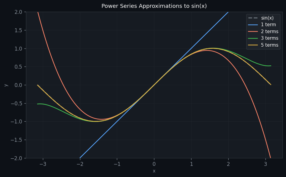
The practical procedure: substitute \( y = \sum_{n=0}^{\infty} a_n x^n \) into the DE, differentiate term by term, and collect like powers of \( x^n \). Setting each coefficient to zero yields a recurrence relation for the \( a_n \).

Notice that \( a_0 \) and \( a_1 \) are the two free parameters — they correspond to the initial conditions \( y(0) = a_0 \) and \( y'(0) = a_1 \).

Hermite’s Equation

The Hermite equation \( y'' - 2xy' + 2\alpha y = 0 \) arises in quantum mechanics. The power series method yields the recurrence

\[ a_{n+2} = \frac{2(n - \alpha)}{(n+2)(n+1)}a_n. \]

When \( \alpha = n \) is a nonnegative integer, one of the two series terminates, yielding the Hermite polynomials \( H_n(x) \). For non-integer \( \alpha \), both series have infinite radius of convergence but grow too rapidly to be physically useful.

---

Chapter 4: Series Solutions — The Frobenius Method

Regular Singular Points

When the standard-form coefficients \( P(x) \) or \( Q(x) \) fail to be analytic at \( x_0 \), we call \( x_0 \) a singular point. A singular point \( x_0 \) is regular if the limits

\[ \lim_{x \to x_0}(x - x_0)P(x) \quad \text{and} \quad \lim_{x \to x_0}(x - x_0)^2 Q(x) \]

both exist (and are finite). Otherwise it is an irregular singular point.

The Frobenius Method: Power Series with Unknown Exponent

At a regular singular point \( x_0 = 0 \), we seek solutions of the form

\[ y(x) = x^r \sum_{n=0}^{\infty} a_n x^n = \sum_{n=0}^{\infty} a_n x^{n+r}, \qquad a_0 \neq 0, \]

where the indicial exponent \( r \) is to be determined. Substituting into the original DE (before dividing by \( x^2 \)) and collecting the lowest power of \( x \) yields the indicial equation:

\[ r(r-1) + p_0 r + q_0 = 0, \]

where \( p_0 = \lim_{x \to 0} xP(x) \) and \( q_0 = \lim_{x \to 0} x^2 Q(x) \). This is a quadratic in \( r \) with roots \( r_1 \geq r_2 \) (assuming \( r_1 - r_2 \geq 0 \)).

The Three Cases

The nature of the second linearly independent solution depends on the difference \( r_1 - r_2 \):

\[ y_1(x) = x^{r_1}\sum_{n=0}^{\infty}a_n x^n, \qquad y_2(x) = x^{r_2}\sum_{n=0}^{\infty}b_n x^n. \]\[ y_2(x) = y_1(x)\ln x + x^{r_1}\sum_{n=1}^{\infty}c_n x^n. \]\[ y_2(x) = Cy_1(x)\ln x + x^{r_2}\sum_{n=0}^{\infty}d_n x^n. \]

Bessel’s Equation of Order \( \nu \)

The Bessel equation of order \( \nu \) is

\[ x^2 y'' + xy' + (x^2 - \nu^2)y = 0. \]

The indicial equation is \( r^2 - \nu^2 = 0 \), giving roots \( r_1 = \nu \) and \( r_2 = -\nu \). The Frobenius solution for \( r_1 = \nu \) is the Bessel function of the first kind:

\[ J_\nu(x) = \sum_{m=0}^{\infty} \frac{(-1)^m}{m!\,\Gamma(m+\nu+1)}\left(\frac{x}{2}\right)^{2m+\nu}. \]

For non-integer \( \nu \), \( J_{-\nu}(x) \) is the second linearly independent solution. For integer \( n \), however, \( J_{-n} = (-1)^n J_n \), and the second solution is the Bessel function of the second kind \( Y_n(x) \), which involves a logarithm and is singular at \( x = 0 \).

Some important values and properties:

• \( J_0(0) = 1 \), \( J_n(0) = 0 \) for \( n \geq 1 \)
• \( J_\nu'(x) = \frac{1}{2}[J_{\nu-1}(x) - J_{\nu+1}(x)] \) (recurrence relation)
• Both \( J_\nu \) and \( Y_\nu \) have infinitely many positive zeros, densely packed as \( x \to \infty \)
• The asymptotic behaviour for large \( x \): \( J_\nu(x) \approx \sqrt{2/(\pi x)}\cos(x - \nu\pi/2 - \pi/4) \)

For the special case \( \nu = 1/2 \), the Bessel equation reduces (after the substitution \( y = u/\sqrt{x} \)) to \( u'' + u = 0 \), giving

\[ J_{1/2}(x) = \sqrt{\frac{2}{\pi x}}\sin x, \qquad J_{-1/2}(x) = \sqrt{\frac{2}{\pi x}}\cos x. \]

---

Chapter 5: Qualitative Analysis and Oscillation Theory

Reduction to Normal Form

Any homogeneous second-order linear ODE

\[ y'' + P(x)y' + Q(x)y = 0 \]

can be transformed to the normal form without a first-derivative term via the substitution

\[ y(x) = e^{-\frac{1}{2}\int P(x)\,dx}\,u(x), \]

which yields

\[ u'' + q(x)u = 0, \qquad q(x) = Q(x) - \frac{1}{2}P'(x) - \frac{1}{4}P(x)^2. \]

Since the exponential prefactor is never zero, zeros of \( u(x) \) are in one-to-one correspondence with zeros of \( y(x) \). The qualitative analysis of the original DE can therefore be carried out on the simpler equation \( u'' + q(x)u = 0 \).

For Bessel’s equation, \( P = 1/x \) gives \( \alpha(x) = 1/\sqrt{x} \), and the normal form is

\[ u'' + \left(1 - \frac{1 - 4p^2}{4x^2}\right)u = 0. \]

As \( x \to \infty \), \( q(x) \to 1 \), so Bessel functions behave asymptotically like \( (c_1\cos x + c_2\sin x)/\sqrt{x} \) — oscillatory with amplitude decaying as \( 1/\sqrt{x} \).

Nonoscillatory Solutions: \( q(x) < 0 \)

This explains why, for example, the solutions to \( y'' - y = 0 \) (i.e., \( e^x \) and \( e^{-x} \)) have at most one zero on \( \mathbb{R} \).

Oscillatory Solutions: The Integral Condition

The proof proceeds by contradiction: if \( u \) has only finitely many zeros, one can define \( v = -u'/u \) and integrate \( v' = q(x) + v^2 \) to show \( v \) must become positive and grow without bound, forcing \( u' < 0 \) and eventually \( u < 0 \), a contradiction.

Examples:

1. \( u'' + u = 0 \): \( q = 1 \), \( \int_1^\infty dx = \infty \). All nontrivial solutions are oscillatory. ✓
2. Bessel’s equation, normal form: \( q(x) = 1 - (1-4p^2)/(4x^2) \), \( \int_1^\infty q\,dx = \infty \). All Bessel functions \( J_p(x) \) and \( Y_p(x) \) have infinitely many positive zeros.
3. Euler-Cauchy type \( u'' + c x^{-2}u = 0 \) for \( c > 1/4 \): still oscillatory. For \( c \leq 1/4 \): not oscillatory.

The Sturm Separation Theorem

This reflects the fact that for a two-dimensional solution space, the zero-sets of linearly independent solutions must interlace.

The Sturm Comparison Theorem

Intuitively: the “stronger restoring force” in \( q_2 \) causes \( v \) to oscillate at least as rapidly as \( u \). If \( q_2 > q_1 \), then \( v \) oscillates strictly more rapidly. This gives a rigorous formulation of the heuristic observation in Chapter 1 about solutions to \( y'' + (1+x)y = 0 \) oscillating faster than those of \( y'' + y = 0 \).

---

Chapter 5 (cont’d): Zeros of Bessel Functions and the Vibrating Drum

Zeros of Bessel Functions

Since \( \int_1^\infty q(x)\,dx = \infty \) for Bessel’s normal form, all Bessel functions have infinitely many positive zeros. Let \( x_{m,k} \) denote the \( k \)-th positive zero of \( J_m(x) \). The Sturm Comparison theorem applied to the normal form shows that consecutive zeros are separated by approximately \( \pi \) for large \( x \), reflecting the asymptotic oscillatory behaviour.

Key zeros of \( J_0 \): \( x_{0,1} \approx 2.4048 \), \( x_{0,2} \approx 5.5201 \), \( x_{0,3} \approx 8.6537 \), \ldots

The Vibrating Circular Drum

The vibrations of a thin elastic circular membrane of radius \( R_0 \) are governed by the two-dimensional wave equation

\[ \frac{\partial^2 u}{\partial t^2} = K\nabla^2 u, \qquad K = \frac{T}{\rho}, \]

where \( u(r, \theta, t) \) is the displacement, \( T \) is tension per unit length, and \( \rho \) is the surface mass density. Seeking solutions of the form

\[ u(r, \theta, t) = v(r, \theta)\cos\omega t \]

yields the Helmholtz equation \( \nabla^2 v + a^2 v = 0 \) with \( a^2 = \omega^2/K \). A further separation \( v(r,\theta) = R(r)S(\theta) \) gives:

\[ S(\theta) = c_1\cos(m\theta) + c_2\sin(m\theta), \qquad m = 0, 1, 2, \ldots \]\[ s^2 R'' + sR' + (s^2 - m^2)R = 0, \]

which is exactly Bessel’s equation of order \( m \). Since \( Y_m(s) \to -\infty \) as \( s \to 0^+ \), the requirement of finite displacement at the centre forces

\[ R(s) = c_1 J_m(s). \]

The clamping condition \( u(R_0, \theta, t) = 0 \) requires \( J_m(aR_0) = 0 \), i.e., \( aR_0 = x_{m,k} \). This determines the allowed frequencies:

\[ \omega_{m,k} = \frac{x_{m,k}}{R_0}\sqrt{\frac{T}{\rho}}. \]

Case \( m = 0 \) (radially symmetric modes): The displacement \( u = J_0(ar)\cos\omega t \) is radially symmetric. Choosing \( k = 1 \) (first zero of \( J_0 \)) gives the fundamental frequency \( \omega_{0,1} = (x_{0,1}/R_0)\sqrt{T/\rho} \). In this mode, all points of the membrane move up and down in unison — no nodal circles inside the drum. Higher values of \( k \) introduce \( k - 1 \) nodal circles at radii \( r = (x_{0,j}/x_{0,k})R_0 \) for \( j < k \).

Case \( m = 1 \) (diametric nodal line): Now \( S(\theta) = \cos\theta \), which changes sign across the diameter \( \theta = \pi/2 \). The clamping condition requires \( J_1(aR_0) = 0 \), giving frequencies \( \omega_{1,k} = (x_{1,k}/R_0)\sqrt{T/\rho} \). The first zero of \( J_1 \) is \( x_{1,1} \approx 3.8317 \). Each higher mode adds a nodal circle combined with the diameter.

\[ \omega_{m,k+1} - \omega_{m,k} \to \frac{\pi}{R_0}\sqrt{\frac{T}{\rho}}, \qquad k \to \infty. \]

This is a beautiful connection between the mathematical theory of zeros of Bessel functions, the Sturm Comparison Theorem, and the physics of percussion instruments.

---

Chapter 6: Existence and Uniqueness — Picard’s Theorem

The Scalar IVP as a Fixed-Point Problem

We seek to prove existence and uniqueness for the first-order IVP

\[ y' = f(y, x), \qquad y(x_0) = y_0. \]

The key idea is to reformulate it as an integral equation:

\[ y(x) = y_0 + \int_{x_0}^x f(y(s), s)\,ds. \]

A solution is a fixed point of the Picard operator \( T \), defined by

\[ (Tu)(x) = y_0 + \int_{x_0}^x f(u(s), s)\,ds. \]

The Lipschitz Condition

A sufficient condition: if \( \partial f/\partial y \) is bounded by \( K \) on \( I \), then \( f \) is Lipschitz with constant \( K \). For example, \( f(y,x) = y^2 \) is Lipschitz on bounded intervals but not on all of \( \mathbb{R} \).

Contraction Mapping and Banach’s Fixed Point Theorem

The space \( F \) used here is the space of continuous functions on \( [x_0, x_1] \) with the uniform norm \( d(u, v) = \max_{x_0 \leq x \leq x_1}|u(x) - v(x)| \), which is complete.

Picard’s Existence-Uniqueness Theorem

\[ d_\infty(Tu, Tv) \leq K|x_1 - x_0|\,d_\infty(u, v). \]

Picard Iteration in Practice

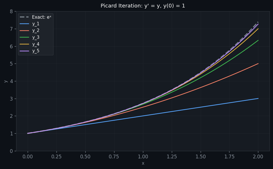
Starting from the initial guess \( u_0(x) = y_0 \), the Picard iterates are

\[ u_{k+1}(x) = y_0 + \int_{x_0}^x f(u_k(s), s)\,ds. \]

Banach’s theorem guarantees that \( u_k \to y \) uniformly, where \( y \) is the unique solution.

Extension to Systems

The above framework extends naturally to the vector IVP \( \mathbf{x}' = \mathbf{f}(\mathbf{x}, t) \), \( \mathbf{x}(t_0) = \mathbf{x}_0 \). The Picard operator becomes vector-valued:

\[ (\mathbf{T}\mathbf{u})(t) = \mathbf{x}_0 + \int_{t_0}^t \mathbf{f}(\mathbf{u}(s), s)\,ds, \]

and a vector Lipschitz condition \( \|\mathbf{f}(\mathbf{x}_1, t) - \mathbf{f}(\mathbf{x}_2, t)\| \leq K\|\mathbf{x}_1 - \mathbf{x}_2\| \) ensures contractivity. This framework proves existence-uniqueness for linear systems with continuous \( A(t) \), which in turn (via the reduction of higher-order DEs to first-order systems) establishes the Existence-Uniqueness theorem for second-order linear DEs stated in Chapter 2.

---

Chapter 7: Linear Systems of ODEs

Reduction to First-Order Systems

Any \( n \)-th order ODE in \( y(t) \) can be rewritten as a first-order system by introducing the variables

\[ x_1 = y, \quad x_2 = y', \quad \ldots, \quad x_n = y^{(n-1)}. \]

The system is then \( \mathbf{x}' = A(t)\mathbf{x} + \mathbf{b}(t) \) for linear equations. For example, the harmonic oscillator \( \ddot{x} + \omega^2 x = 0 \) becomes

\[ \begin{pmatrix} \dot{x}_1 \\ \dot{x}_2 \end{pmatrix} = \begin{pmatrix} 0 & 1 \\ -\omega^2 & 0 \end{pmatrix}\begin{pmatrix} x_1 \\ x_2 \end{pmatrix}. \]

This reformulation serves two purposes: (1) it makes existence-uniqueness theorems easier to prove, and (2) first-order systems are the natural setting for numerical ODE solvers.

The Linear Homogeneous System

We focus on the homogeneous linear system

\[ \mathbf{x}' = A(t)\mathbf{x}, \]

where \( A(t) \) is a continuous \( n \times n \) matrix-valued function on an interval \( I \). The superposition principle holds: any linear combination of solutions is again a solution.

This also proves that the solution space for a scalar second-order linear homogeneous ODE is exactly two-dimensional — a fact stated early in Chapter 2 but now rigorously established.

The Fundamental Matrix

The fundamental matrix is the “propagator” or “flow” of the system: it maps initial conditions to solutions. The Wronskian of the system is the determinant \( W(t) = \det\Phi(t, t_0) \), which satisfies Abel’s identity \( W(t) = \exp\!\left(\int_{t_0}^t \mathrm{tr}(A(s))\,ds\right) \).

Constant Coefficient Systems: The Matrix Exponential

For the autonomous system \( \mathbf{x}' = A\mathbf{x} \) (constant \( A \)), the fundamental matrix is the matrix exponential:

\[ \Phi(t) = e^{tA} = \sum_{k=0}^{\infty}\frac{t^k A^k}{k!} = I + tA + \frac{t^2A^2}{2!} + \cdots \]

This series converges for all \( t \in \mathbb{R} \). The unique solution to the IVP \( \mathbf{x}(0) = \mathbf{a} \) is \( \mathbf{x}(t) = e^{tA}\mathbf{a} \).

Computing \( e^{tA} \) via eigenvalues: If \( A \) has eigenvalues \( \lambda_k \) with eigenvectors \( \mathbf{v}_k \), then \( e^{tA}\mathbf{v}_k = e^{\lambda_k t}\mathbf{v}_k \). For a diagonalizable matrix \( A = PDP^{-1} \):

\[ e^{tA} = Pe^{tD}P^{-1}, \qquad e^{tD} = \mathrm{diag}(e^{\lambda_1 t}, \ldots, e^{\lambda_n t}). \]

Repeated eigenvalues and Jordan form: If \( A \) has a repeated eigenvalue \( \lambda \) with deficient eigenspace (Jordan block), solutions involve terms of the form \( t^k e^{\lambda t} \mathbf{v} \). For the Jordan block \( A = \begin{pmatrix} a & 1 \\ 0 & a \end{pmatrix} \):

\[ e^{tA} = e^{at}\begin{pmatrix} 1 & t \\ 0 & 1 \end{pmatrix}. \]

---

Chapter 8: Phase Portraits and Dynamical Systems

Orbits and the Phase Plane

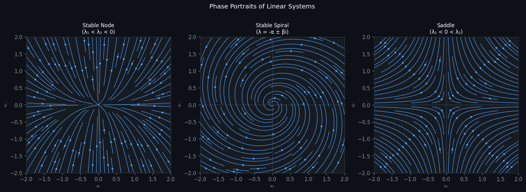
The solutions of the autonomous system \( \mathbf{x}' = A\mathbf{x} \) in \( \mathbb{R}^2 \) can be visualised as orbits — curves traced by \( \mathbf{x}(t) \) in the phase plane as \( t \) varies. The collection of all such orbits constitutes the phase portrait. The origin \( \mathbf{0} \) is always an equilibrium point (fixed point of the flow), since \( A\mathbf{0} = \mathbf{0} \).

The long-time behaviour of solutions is governed by the real parts of the eigenvalues \( \lambda_k \) of \( A \):

\[ e^{at} \to \begin{cases} +\infty & a > 0, \\ 0 & a < 0, \end{cases} \qquad \text{as } t \to \infty. \]

Classification of the Equilibrium at the Origin

For a \( 2 \times 2 \) real matrix \( A \) with eigenvalues \( \lambda_1, \lambda_2 \), the equilibrium \( \mathbf{0} \) is classified by the trace \( \tau = \lambda_1 + \lambda_2 \) and determinant \( \Delta = \lambda_1\lambda_2 \):

Real and distinct eigenvalues (\( \tau^2 > 4\Delta \)):

• Stable node (\( \lambda_1 < \lambda_2 < 0 \)): all orbits approach the origin, tangent to the slower eigenspace. Asymptotically stable.
• Unstable node (\( 0 < \lambda_1 < \lambda_2 \)): all orbits move away from the origin. Unstable.
• Saddle point (\( \lambda_1 < 0 < \lambda_2 \)): the stable manifold (tangent to \( \mathbf{v}_1 \)) approaches the origin; the unstable manifold (tangent to \( \mathbf{v}_2 \)) moves away. Unstable.

Complex eigenvalues \( \lambda = \alpha \pm i\beta \) (\( \tau^2 < 4\Delta \)):

• Stable spiral (\( \alpha < 0 \)): orbits spiral into the origin. Asymptotically stable.
• Unstable spiral (\( \alpha > 0 \)): orbits spiral away. Unstable.
• Centre (\( \alpha = 0 \)): orbits are closed ellipses around the origin. Stable but not asymptotically stable.

Repeated eigenvalue \( \lambda_1 = \lambda_2 = \lambda \):

• Stable star or improper node (\( \lambda < 0 \)): depends on Jordan form. Asymptotically stable.

The Trace-Determinant Plane

The classification can be summarised in the \( (\tau, \Delta) \)-plane. The parabola \( \tau^2 = 4\Delta \) separates spiral/centre types (above) from node/saddle types (below). The \( \Delta > 0 \), \( \tau < 0 \) region corresponds to stable equilibria; \( \Delta > 0 \), \( \tau > 0 \) to unstable; \( \Delta < 0 \) to saddles.

Stable and Unstable Subspaces

For a saddle point, the stable subspace \( E^s \) is spanned by the eigenvectors corresponding to negative eigenvalues, and the unstable subspace \( E^u \) by eigenvectors with positive eigenvalues. Both are invariant under the flow: orbits starting on \( E^s \) approach the origin as \( t \to \infty \), while orbits starting on \( E^u \) approach it as \( t \to -\infty \).

---

Chapter 9: Laplace Transforms

Definition and Basic Transforms

Given a function \( y(t) \), \( t \geq 0 \), its Laplace transform is

\[ Y(s) = \mathcal{L}[y](s) = \int_0^{\infty} e^{-st}y(t)\,dt, \]

defined for all \( s \in \mathbb{C} \) for which the integral converges. The Laplace transform is a linear operator:

\[ \mathcal{L}[c_1 f + c_2 g] = c_1\mathcal{L}[f] + c_2\mathcal{L}[g]. \]

A function is said to be of exponential order \( \alpha \) if \( |f(t)| \leq Ce^{\alpha t} \) for large \( t \). If \( f \) is piecewise continuous and of exponential order \( \alpha \), then \( \mathcal{L}[f](s) \) exists for \( \mathrm{Re}(s) > \alpha \).

Table of standard Laplace transforms:

\( f(t) \)	\( F(s) = \mathcal{L}[f] \)	Conditions
\( 1 \)	\( \dfrac{1}{s} \)	\( \mathrm{Re}(s) > 0 \)
\( e^{at} \)	\( \dfrac{1}{s-a} \)	\( \mathrm{Re}(s) > a \)
\( t^n \)	\( \dfrac{n!}{s^{n+1}} \)	\( \mathrm{Re}(s) > 0 \)
\( \sin bt \)	\( \dfrac{b}{s^2+b^2} \)	\( \mathrm{Re}(s) > 0 \)
\( \cos bt \)	\( \dfrac{s}{s^2+b^2} \)	\( \mathrm{Re}(s) > 0 \)
\( e^{at}\sin bt \)	\( \dfrac{b}{(s-a)^2+b^2} \)	\( \mathrm{Re}(s) > a \)
\( e^{at}\cos bt \)	\( \dfrac{s-a}{(s-a)^2+b^2} \)	\( \mathrm{Re}(s) > a \)
\( H(t-c) \)	\( \dfrac{e^{-cs}}{s} \)	\( \mathrm{Re}(s) > 0 \)

Operational Properties

Differentiation:

\[ \mathcal{L}[f'] = s\mathcal{L}[f] - f(0), \qquad \mathcal{L}[f''] = s^2\mathcal{L}[f] - sf(0) - f'(0). \]

These follow by integration by parts, using \( f(t) = O(e^{\alpha t}) \).

First Shift Theorem: If \( F(s) = \mathcal{L}[f](s) \), then

\[ \mathcal{L}[e^{ct}f(t)] = F(s-c). \]

Second Shift Theorem (Heaviside): With the step function \( H(t-c) = 0 \) for \( t < c \) and \( 1 \) for \( t \geq c \),

\[ \mathcal{L}[H(t-c)f(t-c)] = e^{-cs}F(s). \]

Solving IVPs with Laplace Transforms

The power of the Laplace transform is that it converts an ODE into an algebraic equation. For the IVP

\[ y'' + py' + qy = u(t), \qquad y(0) = y_0, \quad y'(0) = v_0, \]

taking transforms and using the differentiation formulas:

\[ (s^2 + ps + q)Y(s) = U(s) + (s+p)y_0 + v_0. \]

Solving for \( Y(s) \):

\[ Y(s) = \underbrace{\frac{U(s)}{s^2+ps+q}}_{Y_p(s)} + \underbrace{\frac{(s+p)y_0 + v_0}{s^2+ps+q}}_{Y_h(s)}. \]

The first term gives the particular solution (driven by \( u \)); the second gives the homogeneous solution satisfying the initial conditions.

The Transfer Function and Convolution

The transfer function of the linear operator \( L[y] = y'' + py' + qy \) is

\[ G(s) = \frac{1}{s^2 + ps + q}. \]

It describes the system’s response in frequency space: \( Y_p(s) = G(s)U(s) \).

The Convolution Theorem states that

\[ \mathcal{L}^{-1}[F(s)G(s)] = (f * g)(t) = \int_0^t f(t-\tau)g(\tau)\,d\tau. \]

Therefore the particular solution can be written as

\[ y_p(t) = (g * u)(t) = \int_0^t g(t-\tau)u(\tau)\,d\tau, \]

where \( g(t) = \mathcal{L}^{-1}[G(s)] \) is the impulse response (Green’s function) of the system.

---

Chapter 10: The Dirac Delta and Impulsive Forcing

Motivation: Instantaneous Impulses

In many physical applications, a force (or input) acts over an extremely short time interval but delivers a finite total impulse. For example, a bat striking a ball exerts a large force over a tiny time \( \Delta t \), after which the ball’s velocity changes by \( \Delta v = I/m \) where \( I \) is the impulse.

Mathematically, we model such an instantaneous impulse at time \( t = a \) by a sequence of “bump functions” \( f_\Delta(t) \) supported on \( [a, a+\Delta] \) with \( \int f_\Delta\,dt = I \), and take \( \Delta \to 0 \).

The Dirac Delta “Function”

Formally, \( \delta(t-a) \) can be thought of as a limit of spike functions of height \( 1/\Delta \) and width \( \Delta \) centred at \( a \), but it is not a function in the classical sense — it belongs to the theory of distributions.

Laplace transform of \( \delta \):

\[ \mathcal{L}[\delta(t-a)] = e^{-as}, \qquad a > 0. \]

This follows from the sifting property: \( \mathcal{L}[\delta(t-a)] = \int_0^\infty e^{-st}\delta(t-a)\,dt = e^{-as} \).

Solving IVPs with Impulsive Forcing

Systems of DEs with the Laplace Transform

The Laplace transform extends naturally to systems. Taking LTs of \( \mathbf{x}' = A\mathbf{x} + \mathbf{b}(t) \), \( \mathbf{x}(0) = \mathbf{x}_0 \):

\[ (sI - A)\mathbf{X}(s) = \mathbf{x}_0 + \mathbf{B}(s), \]

where \( \mathbf{B}(s) = \mathcal{L}[\mathbf{b}] \). The solution is

\[ \mathbf{X}(s) = (sI - A)^{-1}\mathbf{x}_0 + (sI - A)^{-1}\mathbf{B}(s). \]

The matrix \( (sI - A)^{-1} \) is called the resolvent of \( A \). Its inverse Laplace transform is the fundamental matrix \( \Phi(t) = e^{tA} \):

\[ \mathcal{L}[e^{tA}] = (sI - A)^{-1}. \]

---

Chapter 11: Boundary Value Problems and Eigenvalue Problems

BVPs vs. IVPs: The Key Differences

For initial value problems, the Existence-Uniqueness theorem guarantees exactly one solution for any initial data. For boundary value problems, the situation is fundamentally different: solutions may fail to exist, may be unique, or may be non-unique (infinitely many), depending on the parameter \( \lambda \) in the equation.

Consider the model problem

\[ y'' + \lambda y = 0, \qquad y(0) = 0, \quad y(\pi) = 0. \]

Case \( \lambda < 0 \): The general solution is \( y = c_1 e^{\sqrt{-\lambda}x} + c_2 e^{-\sqrt{-\lambda}x} \), nonoscillatory. The boundary conditions force \( c_1 = c_2 = 0 \); only the trivial solution exists.

Case \( \lambda = 0 \): The general solution is \( y = c_1 + c_2 x \). The boundary conditions force \( c_1 = 0 \) and \( c_2 \pi = 0 \), so again only \( y = 0 \).

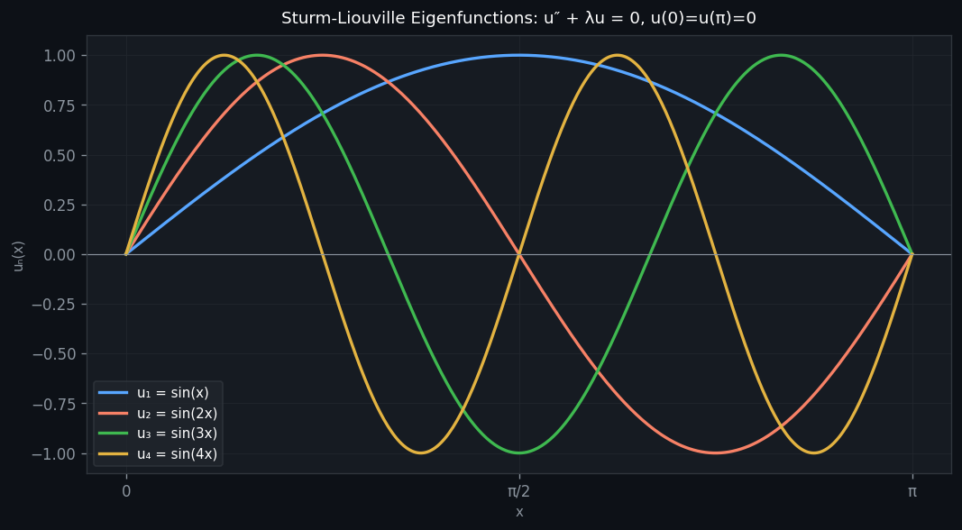
Case \( \lambda > 0 \): The general solution is \( y = c_1\cos\sqrt{\lambda}x + c_2\sin\sqrt{\lambda}x \). The condition \( y(0) = 0 \) gives \( c_1 = 0 \). The condition \( y(\pi) = 0 \) then requires

\[ c_2\sin(\sqrt{\lambda}\,\pi) = 0. \]

For nontrivial solutions, \( \sin(\sqrt{\lambda}\,\pi) = 0 \), which means \( \sqrt{\lambda}\,\pi = n\pi \), i.e., \( \lambda = n^2 \) for \( n = 1, 2, 3, \ldots \).

Eigenvalues and Eigenfunctions

The eigenvalue problem can be written as \( -Ly = \lambda y \) where \( L = d^2/dx^2 \), in analogy with the matrix eigenvalue problem \( A\mathbf{v} = \lambda\mathbf{v} \).

The Vibrating String

The one-dimensional wave equation for a string of length \( L \) clamped at both ends:

\[ \frac{\partial^2 u}{\partial t^2} = K\frac{\partial^2 u}{\partial x^2}, \qquad u(0,t) = u(L,t) = 0. \]

Substituting \( u(x,t) = v(x)\cos\omega t \) yields the eigenvalue problem

\[ v'' + \frac{\omega^2}{K}v = 0, \qquad v(0) = v(L) = 0, \]

with eigenvalues \( \omega_n^2/K = (n\pi/L)^2 \), giving the vibrational frequencies

\[ \omega_n = \frac{n\pi}{L}\sqrt{\frac{T}{\rho}}, \qquad n = 1, 2, 3, \ldots \]

and mode shapes \( v_n(x) = \sin(n\pi x/L) \). The general solution is a superposition:

\[ u(x,t) = \sum_{n=1}^{\infty} c_n \sin\!\left(\frac{n\pi x}{L}\right)\cos(\omega_n t). \]

The coefficients \( c_n \) are determined by the initial displacement \( u(x, 0) = f(x) \), and the key tool for finding them is the orthogonality of the eigenfunctions — the subject of Chapter 12.

---

Chapter 12: Sturm-Liouville Theory

Generalised Eigenvalue Problem

We now consider the more general boundary value/eigenvalue problem:

\[ y'' + \lambda q(x)y = 0, \qquad y(a) = y(b) = 0, \quad q(x) > 0 \text{ on } [a,b]. \]

This arises, for instance, from a vibrating string with variable mass density \( \rho(x) \), where \( q(x) = \rho(x)/T \) plays the role of the weight function.

Orthogonality with Respect to a Weight Function

The Self-Adjoint Operator

The operator \( L = d^2/dx^2 \) restricted to functions vanishing at the boundary is self-adjoint:

\[ \langle Lu, v\rangle = \langle u, Lv\rangle \qquad \text{for all } u, v \in F[a,b], \]

where \( F[a,b] = \{f : [a,b] \to \mathbb{R} \mid f(a) = f(b) = 0\} \). This is proved by double integration by parts:

\[ \int_a^b u''v\,dx = \underbrace{[u'v]_a^b}_{=0} - \int_a^b u'v'\,dx = -\int_a^b u'v'\,dx = \underbrace{[-uv']_a^b}_{=0} + \int_a^b uv''\,dx. \]

The self-adjointness of \( L \) is the functional-analytic reason for the orthogonality of eigenfunctions — precisely analogous to the fact that symmetric matrices have orthogonal eigenvectors.

Generalized Fourier Series and Completeness

The normalised eigenfunctions

\[ \phi_n(x) = \frac{u_n(x)}{\sqrt{N_n}}, \qquad N_n = \langle u_n, u_n\rangle_q = \int_a^b u_n^2 q\,dx, \]

form an orthonormal basis in \( L^2_q[a,b] \): \( \langle\phi_m, \phi_n\rangle_q = \delta_{mn} \). Any function \( f \in L^2_q[a,b] \) can be expanded as

\[ f(x) = \sum_{n=1}^{\infty} c_n u_n(x), \]

where the generalised Fourier coefficients are

\[ c_n = \frac{\langle f, u_n\rangle_q}{N_n} = \frac{\int_a^b f(x)u_n(x)q(x)\,dx}{\int_a^b u_n(x)^2 q(x)\,dx}. \]

The completeness of the eigenfunction expansion is expressed by Parseval’s identity:

\[ \langle f, f\rangle_q = \sum_{n=1}^{\infty} c_n^2 N_n. \]

Partial sums satisfy the Bessel inequality: \( \sum_{n=1}^{N} c_n^2 N_n \leq \langle f, f\rangle_q \).

Generalised Sturm-Liouville Problems

The full Sturm-Liouville operator has the self-adjoint form

\[ Ly = \frac{d}{dx}\left[p(x)\frac{dy}{dx}\right] + r(x)y, \]

and the eigenvalue problem is \( -Ly = \lambda w(x)y \) with appropriate boundary conditions, where \( p(x) > 0 \), \( w(x) > 0 \). The orthogonality of eigenfunctions holds with respect to the weight \( w(x) \):

\[ \int_a^b u_m(x)u_n(x)w(x)\,dx = 0 \quad (m \neq n). \]

Bessel’s equation is an example: with \( p(x) = x \) and \( w(x) = x \), the Bessel functions \( J_\nu(\lambda_k x) \) corresponding to different zeros \( \lambda_k \) of \( J_\nu \) are orthogonal on \( [0, R] \) with weight \( x \). This orthogonality underlies the Fourier-Bessel expansions used in the vibrating drum problem of Chapter 5.

---

Chapter 13: Perturbation Methods

Regular Perturbation and Secular Terms

Many nonlinear ODEs depend on a small parameter \( \epsilon \), e.g.,

\[ y'' + y = \epsilon f(y, y'), \qquad |\epsilon| \ll 1. \]

Regular perturbation assumes a power series in \( \epsilon \):

\[ y(t) = y_0(t) + \epsilon y_1(t) + \epsilon^2 y_2(t) + \cdots \]

Substituting and collecting powers of \( \epsilon \) yields a hierarchy of linear DEs:

\[ y_0'' + y_0 = 0, \qquad y_1'' + y_1 = f(y_0, y_0'), \qquad \ldots \]

The leading-order solution satisfying \( y(0) = A \), \( y'(0) = 0 \) is \( y_0 = A\cos t \).

The secular term problem: When \( f(y_0, y_0') \) contains terms resonant with the homogeneous solution (e.g., \( \cos t \) or \( \sin t \)), the particular solution to the next equation contains terms like \( t\sin t \) or \( t\cos t \). These are called secular terms — they grow without bound as \( t \to \infty \), which is physically nonsensical for a bounded oscillator. The regular perturbation expansion breaks down for \( t = O(1/\epsilon) \).

The Poincaré-Lindstedt Method

The remedy is to allow the frequency of the oscillation to depend on \( \epsilon \) as well. Define a scaled time

\[ s = \omega(\epsilon) t, \qquad \omega(\epsilon) = 1 + \omega_1\epsilon + \omega_2\epsilon^2 + \cdots, \]

and expand \( x \) as a power series in \( \epsilon \) using \( s \) as the variable. The unknown frequency corrections \( \omega_1, \omega_2, \ldots \) are chosen precisely to eliminate secular terms at each order.

The Duffing Oscillator

The Duffing equation models a nonlinear spring:

\[ m\frac{d^2x}{dt^2} + kx + \gamma x^3 = 0. \]

If \( \gamma > 0 \), the spring is hard (stiffening with displacement); if \( \gamma < 0 \), it is soft (softening). After non-dimensionalisation with \( \tau = \omega_0 t \), \( \omega_0 = \sqrt{k/m} \), and \( \epsilon = \gamma/k \):

\[ \frac{d^2x}{d\tau^2} + x + \epsilon x^3 = 0. \]

This is conservative with potential energy \( V(x) = \frac{1}{2}x^2 + \frac{\epsilon}{4}x^4 \), and solutions are periodic (for small \( |\epsilon| \)).

We seek the solution with initial conditions \( x(0) = A \), \( x'(0) = 0 \) (mass released from rest at amplitude \( A \)).

Applying the Poincaré-Lindstedt method:

Let \( s = \omega(\epsilon)\tau \). In terms of \( s \):

\[ \omega^2 x'' + x + \epsilon x^3 = 0 \qquad (' = d/ds). \]

Substitute \( \omega = 1 + \omega_1\epsilon + \cdots \) and \( x = x_0 + \epsilon x_1 + \cdots \):

\[ x_0'' + x_0 = 0, \qquad x_0(0) = A, \quad x_0'(0) = 0 \implies x_0(s) = A\cos s. \]\[ x_1'' + x_1 = -2\omega_1 x_0'' - x_0^3 = 2\omega_1 A\cos s - A^3\cos^3 s. \]

Using the identity \( \cos^3 s = \frac{3}{4}\cos s + \frac{1}{4}\cos 3s \):

\[ x_1'' + x_1 = A\!\left(2\omega_1 - \frac{3A^2}{4}\right)\cos s - \frac{A^3}{4}\cos 3s. \]

The coefficient of \( \cos s \) on the right is a resonant term that would produce secular growth \( \sim s\sin s \). Setting it to zero:

\[ \omega_1 = \frac{3A^2}{8}. \]

The remaining equation

\[ x_1'' + x_1 = -\frac{A^3}{4}\cos 3s \]

has the particular solution \( x_{1,p} = \frac{A^3}{32}\cos 3s \). Imposing \( x_1(0) = 0 \), \( x_1'(0) = 0 \):

\[ x_1(s) = \frac{A^3}{32}(\cos 3s - \cos s). \]

The first-order Poincaré-Lindstedt solution:

\[ x(\tau) = A\cos(\nu\tau) + \frac{\epsilon A^3}{32}[\cos(3\nu\tau) - \cos(\nu\tau)] + O(\epsilon^2), \]

where the nonlinear frequency is

\[ \nu = \omega_0\omega = \omega_0\!\left(1 + \frac{3A^2}{8}\epsilon + O(\epsilon^2)\right) = \sqrt{\frac{k}{m}}\!\left(1 + \frac{3A^2\gamma}{8k} + \cdots\right). \]

The period of oscillation is

\[ T = \frac{2\pi}{\nu} \approx \frac{2\pi}{\omega_0}\left(1 - \frac{3A^2\gamma}{8k}\right). \]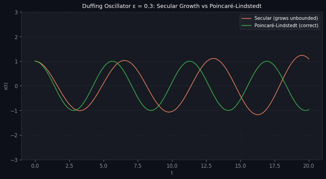

Physical interpretation:

• For a hard spring (\( \gamma > 0 \), \( \epsilon > 0 \)): \( \nu > \omega_0 \), so the frequency increases with amplitude. Larger oscillations are faster. The period is shorter.
• For a soft spring (\( \gamma < 0 \), \( \epsilon < 0 \)): \( \nu < \omega_0 \), so the frequency decreases with amplitude. Larger oscillations are slower. The period is longer.

This amplitude-frequency dependence is a hallmark of nonlinear oscillators and is entirely absent in the linear case (\( \gamma = 0 \)), where the period \( T = 2\pi/\omega_0 \) is independent of amplitude. The Poincaré-Lindstedt method successfully captures this nonlinear effect while remaining uniformly valid for \( t = O(1/\epsilon) \) — far beyond the breakdown of naive regular perturbation.

---

Summary of Key Results

The following table connects the major themes of this course:

Topic	Key Result	Chapter
Linear homogeneous ODE	Solution space is 2-dimensional	2, 7
Wronskian	\( W \equiv 0 \) iff solutions linearly dependent	2
Abel’s Theorem	\( W(x) = Ce^{-\int P\,dx} \)	2
Ordinary points	Power series solutions with radius \( \geq R \)	3
Regular singular points	Frobenius method, indicial equation	4
Bessel functions	\( J_\nu \) from Frobenius with \( r = \nu \)	4
Oscillation theory	\( q > 0 \) and \( \int q = \infty \Rightarrow \) infinitely many zeros	5
Sturm Comparison	Greater \( q \Rightarrow \) more rapid oscillation	5
Vibrating drum	Frequencies from zeros of \( J_m \)	5
Picard theorem	Lipschitz \( + \) contraction \( \Rightarrow \) unique solution	6
Fundamental matrix	\( \Phi(t,t_0) \) maps ICs to solutions, \( \Phi(t_0,t_0) = I \)	7
Matrix exponential	\( e^{tA} \) gives solution to \( \mathbf{x}' = A\mathbf{x} \)	7
Phase portraits	Classified by eigenvalues of \( A \)	8
Laplace transforms	ODE \( \to \) algebraic equation in \( s \)	9
Convolution theorem	\( \mathcal{L}[f*g] = F(s)G(s) \)	9
Dirac delta	\( \mathcal{L}[\delta(t-a)] = e^{-as} \)	10
Eigenvalue problems	Discrete spectrum from BCs	11
Sturm-Liouville	Self-adjoint operator, orthogonal eigenfunctions	12
Parseval’s identity	\( \|f\|^2 = \sum c_n^2 N_n \)	12
Poincaré-Lindstedt	Frequency depends on amplitude for nonlinear oscillator	13