Partial Differential Equations II picks up where the first course left off and pursues two intertwined goals: to develop a geometric and analytical framework for understanding all PDEs, and then to apply that framework systematically to the three great classical equations — Laplace’s, the wave equation, and the heat equation. The course opens with a tour of first-order theory, where the method of characteristics converts a PDE into an equivalent family of ODEs and makes the geometry of solutions vivid. It then classifies second-order equations by the sign of a single discriminant, revealing why Laplace’s equation behaves so differently from the wave equation. The bulk of the course treats each type in turn: elliptic equations through harmonic function theory, maximum principles, Green’s functions, and conformal mapping; hyperbolic equations through d’Alembert’s formula and spherical means; parabolic equations through eigenfunction expansions and the Fourier transform.

Part I: First-Order PDEs and Classification

Chapter 1: The Cauchy Problem and Method of Characteristics

From ODEs to PDEs

The starting point is a familiar ODE:

\[ u_t = F(t, u), \quad u(0) = u_0. \]

When \(F\) is continuous in \(t\) and Lipschitz continuous in \(u\), the Picard–Lindelöf theorem guarantees a unique local solution. This solution may exist globally or may blow up in finite time. Now suppose \(u\), \(F\), and \(u_0\) all depend on a spatial variable \(x\). Then \(u = u(x,t)\) solves a PDE:

\[ \begin{cases} u_t = F(x, t, u), \\ u(x,0) = u_0(x). \end{cases} \]

When \(F\) and \(u_0\) are continuous in \(x\), so is the solution. Geometrically, the graph of \(u\) is a surface in \((x,t,u)\)-space containing the initial curve \(\Gamma_0 = \{(x, 0, u_0(x))\}\). The surface may be smooth for all \(t > 0\), or it may develop a fold or singularity — a phenomenon that depends on \(x\).

This geometric picture motivates the method of characteristics, which applies to the general first-order quasi-linear PDE.

Method of Characteristics

Consider the transport equation as a first illustration:

\[ \text{(P1)} \quad \begin{cases} u_t + a u_x = 0, \\ u(x,0) = h(x), \end{cases} \]

where \(a\) is a constant. We look for a curve \(x = x(t)\) along which \(u\) is constant. By the chain rule,

\[ \frac{d}{dt} u(x(t), t) = u_t + \dot{x} u_x. \]

For this to equal zero — that is, for \(u\) to be constant along the curve — we need \(\dot{x} = a\), giving the characteristic curves \(x = at + x_0\). Along each such line, \(u_t + au_x = 0\) holds, so \(u\) equals its initial value \(h(x_0) = h(x - at)\). The solution is thus

\[ u(x,t) = h(x-at), \]

the initial data “transported” rigidly at speed \(a\) without change of shape.

Characteristic lines for the transport equation \(u_t + a u_x = 0\): each line carries the initial value \(h(x_0)\) rigidly to the right at speed \(a\).

Now consider a general first-order quasi-linear PDE in two independent variables:

\[ \text{(P2)} \quad a(x,y,u)\, u_x + b(x,y,u)\, u_y = c(x,y,u), \]

where \(x,y\) are independent variables, \(u = u(x,y)\) is unknown, and \(a,b,c\) are given smooth functions. The equation is semi-linear if \(a,b\) are independent of \(u\), and linear if in addition \(c\) is linear in \(u\).

The graph \(z = u(x,y)\) in \(\mathbb{R}^3\) has normal vector \(\mathbf{n}_0 = (-u_x, -u_y, 1)\). From (P2), the vector field \(V = (a, b, c)\) is perpendicular to \(\mathbf{n}_0\) everywhere on the graph. Therefore the graph must be tangent to \(V\) at each point — it is an integral surface of the vector field \(V = (a,b,c)\).

The characteristics satisfy the characteristic ODEs:

\[ \frac{dx}{dt} = a(x,y,u), \quad \frac{dy}{dt} = b(x,y,u), \quad \frac{dz}{dt} = c(x,y,u), \]

which can be written in the symmetric form \(dx/a = dy/b = du/c\). Since \(a,b,c\) are \(C^1\), these ODEs can be solved locally for small \(|t - t_0|\). Crucially, any smooth union of characteristics is an integral surface of \(V\), and therefore solves (P2).

The Cauchy Problem

Given a curve \(\Gamma \subset \mathbb{R}^3\), the Cauchy Problem asks for a solution \(z = u(x,y)\) of (P2) whose graph contains \(\Gamma\). Parameterize \(\Gamma\) as:

\[ \Gamma: \quad x = f(s),\; y = g(s),\; z = h(s), \quad s \in I. \]

We launch a characteristic from each point of \(\Gamma\) with initial conditions \(x(s,0) = f(s)\), \(y(s,0) = g(s)\), \(u(s,0) = h(s)\). This generates an integral surface parameterized by \((s,t)\). To recover \(u(x,y)\) we must invert \((s,t) \mapsto (x(s,t), y(s,t))\), which by the inverse function theorem requires the Jacobian to be non-zero:

\[ \det \begin{bmatrix} x_s & y_s \\ x_t & y_t \end{bmatrix} = \det \begin{bmatrix} f'(s) & g'(s) \\ a(f,g,h) & b(f,g,h) \end{bmatrix} \neq 0. \tag{**} \]

Geometrically, this says the projection of \(\Gamma\) onto the \(xy\)-plane is nowhere parallel to the vector field \((a,b)\). Condition \((**)\) is the non-characteristic condition: \(\Gamma\) is non-characteristic for the PDE. When it holds, there exists a unique solution near \(\Gamma\).

Theorem (Local Existence). If \(\Gamma\) is non-characteristic for (P2) and \(a, b, c \in C^1\), then there exists a unique \(C^1\) solution of the Cauchy Problem in a neighborhood of \(\Gamma\).

Example. Solve \(u_t + u\, u_x = 1\) with \(u(x,0) = x\). The characteristic equations are \(dt/d\tau = 1\), \(dx/d\tau = u\), \(du/d\tau = 1\). With \(\Gamma: (0, s, s)\), we get \(t = \tau\), \(u = \tau + s\), and \(x = \frac{1}{2}\tau^2 + s\tau + s\). Solving for \(s\) gives \(s = (x - \frac{1}{2}t^2)/(1+t)\), so

\[ u(x,t) = \frac{x + t + \frac{1}{2}t^2}{1+t}. \]

First Integrals and the General Solution

An alternative approach to finding the general solution of (P2) uses first integrals. A function \(f(x,y,u)\) is a first integral of the characteristic ODEs if it is constant along every characteristic. If we can identify two independent first integrals \(f(x,y,u) = C_1\) and \(g(x,y,u) = C_2\), then the general solution of (P2) is:

\[ f(x,y,u) = F\bigl(g(x,y,u)\bigr), \]

where \(F\) is an arbitrary function, determined by imposing Cauchy data.

Example. For \(u_t + u\, u_x = 1\) (the Burgers-type equation), written symmetrically as \(dt/1 = dx/u = du/1\), one sees \(u - t = \text{const}\) (from the first and third ratios) and then \(x - \frac{1}{2}u^2 + \frac{1}{2}t^2 - tu = \text{const}\). These yield the implicit general solution.

Generalization to \(n\) Independent Variables and Semi-Linear PDEs

The first-order framework extends to \(n\) independent variables:

\[ \sum_{i=1}^n a_i(x_1, \ldots, x_n, u)\, \frac{\partial u}{\partial x_i} = c(x_1, \ldots, x_n, u). \]

The characteristics are integral curves of the \((n+1)\)-dimensional vector field \((a_1, \ldots, a_n, c)\), satisfying \(n+1\) ODEs. Initial data is prescribed on an \((n-1)\)-dimensional manifold, and the non-characteristic Jacobian condition determines when a unique solution exists.

For semi-linear PDEs of general order \(k\):

\[ \left(\sum_{|\alpha|=k} a_\alpha(x)\, D^\alpha u\right) + a_0(x, u, Du, \ldots, D^{k-1}u) = 0, \]

the multi-index notation \(\alpha = (\alpha_1, \ldots, \alpha_n) \in \mathbb{N}^n\), \(|\alpha| = \alpha_1 + \cdots + \alpha_n\), and \(D^\alpha = (\partial/\partial x_1)^{\alpha_1} \cdots (\partial/\partial x_n)^{\alpha_n}\) organizes the higher-order terms compactly.

The Cauchy–Kowalevski Theorem

In the analytic setting, the Cauchy–Kowalevski theorem provides a definitive existence result: if the coefficients and initial data are real-analytic and the initial hypersurface is non-characteristic, then a unique real-analytic solution exists locally. This is the PDE analogue of the ODE theorem on power-series solutions. However, the theorem says nothing about non-analytic data, and more seriously, it does not guarantee well-posedness in the sense of stability — even analytic initial data can lead to unstable solutions for certain PDE types (most famously, the Cauchy problem for the Laplace equation is ill-posed in this sense).

---

Chapter 2: Classification of Second-Order PDEs and Well-Posedness

The Discriminant and PDE Type

The most important second-order linear PDE in two variables is:

\[ \text{(*)} \quad a(x,y)\, u_{xx} + b(x,y)\, u_{xy} + c(x,y)\, u_{yy} = d(x,y,u,u_x,u_y). \]

Given Cauchy data along a curve \(\gamma: (f(s), g(s))\) in the \(xy\)-plane,

\[ u|_\gamma = h(s), \quad \frac{\partial u}{\partial n}\bigg|_\gamma = h_1(s), \]

one asks: when does this data uniquely determine \(u_{xx}\), \(u_{xy}\), \(u_{yy}\) along \(\gamma\)? Differentiating the Cauchy data along \(\gamma\) and using (*) leads to a linear system. The system fails to have a unique solution precisely when

\[ a(g')^2 - b(f')(g') + c(f')^2 = 0. \tag{\star} \]

This is the characteristic condition, and \(\gamma\) is characteristic for (*) when \((\star)\) holds.

The principal symbol of (*) is

\[ \sigma(\xi) = \sigma(x,y;\xi) = a(x,y)\,\xi_1^2 + b(x,y)\,\xi_1\xi_2 + c(x,y)\,\xi_2^2, \]

where \(\xi = (\xi_1, \xi_2)\). The curve \(\gamma\) is characteristic at \((x,y)\) if and only if \(\sigma\) vanishes on the normal \((g', -f')\) to \(\gamma\). Writing the characteristic condition as \(a\,dy^2 - b\,dx\,dy + c\,dx^2 = 0\) and solving for \(dy/dx\):

\[ \frac{dy}{dx} = \frac{b \pm \sqrt{b^2 - 4ac}}{2a}. \]

The sign of the discriminant \(b^2 - 4ac\) determines the PDE type:

The prototypes are: the wave equation \(u_{xx} - u_{yy} = 0\) (hyperbolic, \(b^2-4ac = 4 > 0\)); the heat equation \(u_{xx} - u_t = 0\) (parabolic, \(b^2-4ac = 0\)); and Laplace’s equation \(u_{xx} + u_{yy} = 0\) (elliptic, \(b^2 - 4ac = -4 < 0\)).

PDE classification by discriminant: hyperbolic equations (wave) propagate along two characteristic families; parabolic equations (heat) along one; elliptic equations (Laplace) have no real characteristics and are solved as boundary-value problems.

The Tricomi equation \(u_{yy} - y u_{xx} = 0\) changes type depending on \(y\): it is elliptic for \(y < 0\), parabolic on \(y = 0\), and hyperbolic for \(y > 0\).

Canonical Forms

A change of variables \((x,y) \mapsto (\xi, \eta)\) can simplify the principal part. For a hyperbolic equation, the two families of characteristic curves \(\xi(x,y) = \text{const}\) and \(\eta(x,y) = \text{const}\) define coordinates in which the equation takes the canonical form \(u_{\xi\eta} + \text{lower order}\). For a parabolic equation, one family of characteristics defines one coordinate and the canonical form is \(u_{\xi\xi} + \text{lower order}\). For an elliptic equation, using complex characteristics leads to the canonical form \(u_{\xi\xi} + u_{\eta\eta} + \text{lower order}\).

First-Order Systems

Second-order equations can often be rewritten as first-order systems, which is natural for numerical methods and theoretical analysis. For example, the wave equation \(u_{xx} - u_{yy} = 0\) becomes, with \(u_1 = u_x\) and \(u_2 = u_y\):

\[ \begin{pmatrix} u_1 \\ u_2 \end{pmatrix}_y + \begin{pmatrix} 0 & -1 \\ -1 & 0 \end{pmatrix} \begin{pmatrix} u_1 \\ u_2 \end{pmatrix}_x = \begin{pmatrix} 0 \\ 0 \end{pmatrix}. \]

For a general \(n \times n\) first-order system

\[ \text{(*)} \quad \mathbf{u}_t + A(x,t)\,\mathbf{u}_x = \mathbf{c}(x,t,\mathbf{u}), \]

a curve \(\gamma: (x(t), t)\) is characteristic if \(\det\bigl(I\,\dot{x} - A\bigr) = 0\), that is, if \(\dot{x} = \lambda(x,t)\) where \(\lambda\) is an eigenvalue of \(A\). The principal symbol is the matrix \(\sigma(\xi) = A\,\xi_1 + I\,\xi_2\).

The system (*) is classified by the eigenstructure of \(A\):

For a hyperbolic system, one can diagonalize: let \(P = (\mu_1, \ldots, \mu_n)\) be the matrix of eigenvectors and \(\Lambda = \text{diag}(\lambda_1,\ldots,\lambda_n)\), so \(P^{-1}AP = \Lambda\). Setting \(\mathbf{v} = P^{-1}\mathbf{u}\) transforms (*) into

\[ \mathbf{v}_t + \Lambda\,\mathbf{v}_x = \tilde{\mathbf{c}}(x,t,\mathbf{v}), \]

where \(\tilde{\mathbf{c}} = P^{-1}(\mathbf{c} - P_t\mathbf{v} - AP_x\mathbf{v})\). In the linear case this decouples into \(n\) independent transport equations, each propagating along one family of characteristics.

Well-Posedness

A PDE problem is well-posed in the sense of Hadamard (1923) if:

1. a solution exists;
2. the solution is unique;
3. the solution depends continuously on the data (stability).

Well-posedness is not automatic. The Dirichlet problem for Laplace’s equation — prescribing \(u\) on the boundary of a domain — is well-posed. But the Cauchy problem for Laplace’s equation (prescribing both \(u\) and its normal derivative on a curve) is ill-posed: by Hadamard’s example, arbitrarily small perturbations in the data can cause arbitrarily large changes in the solution. This failure reflects the elliptic character of Laplace’s equation — it has no real characteristics, and therefore information cannot be prescribed on a characteristic in the usual sense. The appropriate boundary conditions depend fundamentally on the PDE type.

---

Part II: Elliptic Equations

Chapter 3: Harmonic Functions and Green’s Identities

Laplace and Poisson Equations

The prototype elliptic equations are:

\[ \Delta u = 0 \quad \text{in } \Omega \subset \mathbb{R}^n \tag{1} \]\[ \Delta u = f \quad \text{in } \Omega \subset \mathbb{R}^n \tag{2} \]

known as Laplace’s equation and Poisson’s equation respectively. Here \(\Delta = \nabla^2 = \sum_{i=1}^n \partial^2/\partial x_i^2\) is the Laplacian, and \(\Omega\) is a domain (open, path-connected subset of \(\mathbb{R}^n\)). Solutions of (1) are called harmonic functions and form the central objects of elliptic theory.

The Cauchy problems for (1) and (2) — prescribing both \(u\) and \(\partial u/\partial n\) on a hypersurface — are not well-posed in general. The natural and well-posed problems are instead boundary value problems:

If we wish to solve \(\Delta u = F\) in \(\Omega\) with \(u = g\) on \(\partial\Omega\), we may decompose \(u = u_1 + u_2\) where \(u_1\) solves the Poisson equation with zero boundary data and \(u_2\) solves Laplace’s equation with the given boundary data. This reduces the Dirichlet problem to two simpler problems.

Green’s Identities

The fundamental analytical tool for elliptic equations is integration by parts in the form of Green’s identities. Let \(\Omega \subset \mathbb{R}^n\) be a smooth, bounded domain and let \(u, v \in C^2(\bar{\Omega})\).

First Green’s Identity:

\[ \int_\Omega \bigl(v\,\Delta u + \nabla u \cdot \nabla v\bigr)\,dx = \int_{\partial\Omega} v\,\frac{\partial u}{\partial n}\,dS. \]

Proof: Apply the divergence theorem \(\int_\Omega \nabla \cdot \mathbf{V}\,dx = \int_{\partial\Omega} \mathbf{V} \cdot \mathbf{n}\,dS\) to \(\mathbf{V} = v\,\nabla u\).

Second Green’s Identity:

\[ \int_\Omega \bigl(v\,\Delta u - u\,\Delta v\bigr)\,dx = \int_{\partial\Omega} \left(v\,\frac{\partial u}{\partial n} - u\,\frac{\partial v}{\partial n}\right)dS. \]

This follows from the first identity by exchanging \(u\) and \(v\) and subtracting. Several immediate consequences follow:

• Setting \(v = 1\) in the first identity: \(\int_\Omega \Delta u\,dx = \int_{\partial\Omega} \partial u/\partial n\,dS\). For the Neumann problem \(\Delta u = F\) with \(\partial u/\partial n = f\), this gives the solvability condition: \(\int_\Omega F\,dx = \int_{\partial\Omega} f\,dS\). The data cannot be chosen freely; this is a necessary condition for existence.

• Uniqueness for Dirichlet: If \(u,v\) both solve \(\Delta u = f\) with \(u = v\) on \(\partial\Omega\), then \(w = u - v\) satisfies \(\Delta w = 0\) in \(\Omega\) and \(w = 0\) on \(\partial\Omega\). Setting \(v = w\) in the first identity gives \(\int_\Omega |\nabla w|^2\,dx = 0\), so \(\nabla w \equiv 0\), hence \(w \equiv 0\).

• Uniqueness for Robin: Similar argument; uniqueness holds when \(\alpha \geq 0\).

---

Chapter 4: Maximum Principles and Mean Value Properties

The maximum principle is one of the most powerful results in elliptic theory. It says, informally, that a harmonic function cannot achieve its maximum (or minimum) in the interior of a domain — it must do so on the boundary.

The Mean Value Property

Let \(\Omega \subset \mathbb{R}^n\) be a domain and \(u \in C^2(\Omega)\) be harmonic. For any point \(\xi \in \Omega\) and any ball \(B(\xi; r) \subset\subset \Omega\), define the spherical mean:

\[ M_u(\xi; r) = \frac{1}{A(\xi,1)} \int_{|\mathbf{x}|=1} u(\xi + r\mathbf{x})\,dS, \]

the average of \(u\) over the sphere of radius \(r\) centered at \(\xi\) (here \(A(\xi,1)\) is the surface area of the unit sphere).

Proof. Using the first Green’s identity with \(v = 1\) and \(\Delta u = 0\) in \(\Omega\):

\[ 0 = \int_{B(\xi,r)} \Delta u\,dx = \int_{\partial B(\xi,r)} \frac{\partial u}{\partial n}\,dS. \]

Changing variables \(\xi' = \xi + r\mathbf{x}\) and differentiating with respect to \(r\) shows that \(\partial M_u(\xi;r)/\partial r = 0\), so \(M_u(\xi;r)\) is independent of \(r\). By continuity, \(M_u(\xi;r) \to u(\xi)\) as \(r \to 0^+\), so the mean equals \(u(\xi)\) for all \(r\). \(\square\)

A function \(u \in C^0(\Omega)\) satisfying the mean value property is said to have the MVP. Remarkably, the MVP implies harmonicity: if \(u \in C^2(\Omega)\) has the MVP, then \(\Delta u = 0\). The MVP also has a volume version: integrating over \(\rho \in [0,r]\) yields

\[ u(\xi) = \frac{1}{V(\xi;1)} \int_{|\mathbf{x}| \leq 1} u(\xi + r\mathbf{x})\,dx. \]

Subharmonic Functions and Weak Maximum Principle

A function \(u \in C^2(\Omega)\) is subharmonic if \(\Delta u \geq 0\) in \(\Omega\). For subharmonic \(u\), the spherical mean \(M_u(\xi;r)\) is increasing in \(r\) (since \(\partial M_u/\partial r \geq 0\) by the same calculation above), so

\[ u(\xi) \leq M_u(\xi;r). \]

This one inequality is the seed of the maximum principle.

Proof (in two steps). Step 1: Suppose strictly \(\Delta u > 0\). If \(u\) achieves its maximum at an interior point \(\xi\), then at \(\xi\) all second derivatives \(u_{x_i x_i} \leq 0\), giving \(\Delta u(\xi) \leq 0\), a contradiction. So the max is on \(\partial\Omega\).

Step 2: For the general case \(\Delta u \geq 0\), let \(v = u - kt\) for small \(k > 0\). Then \(\Delta v = \Delta u - k \cdot 0 = \Delta u \geq 0\)… but actually, the standard approach is: set \(v = u - k|x|^2\) for small \(k > 0\). Then \(\Delta v = \Delta u - 2kn \geq -2kn\). Actually the direct approach: set \(v_k = u + k e^{x_1}\). Then \(\Delta v_k = \Delta u + k e^{x_1} > 0\). By Step 1, \(\max_{\bar\Omega} v_k = \max_{\partial\Omega} v_k\), so \(\max_{\bar\Omega} u \leq \max_{\bar\Omega} v_k = \max_{\partial\Omega} v_k \leq \max_{\partial\Omega} u + k \max_{\partial\Omega} e^{x_1}\). Letting \(k \to 0^+\) gives the result. \(\square\)

Strong Maximum Principle: If \(\Omega\) is connected and \(u\) achieves its maximum at an interior point, then \(u \equiv \text{const}\) in \(\Omega\). This follows from the subharmonic mean-value inequality: if \(u(\xi) = A^* = \sup_\Omega u\) at an interior point, then by the volume MVP, \(u = A^*\) on an entire ball around \(\xi\), and path-connectedness propagates this throughout \(\Omega\).

---

Chapter 5: Green’s Functions and Integral Representations

The Fundamental Solution of the Laplacian

Rather than solving specific BVPs directly, one seeks a single fundamental solution — a “kernel” from which all solutions can be built. We want \(K(x)\) satisfying

\[ \Delta K = \delta(x) \quad \text{in } \mathbb{R}^n, \]

where \(\delta\) is the Dirac delta. Since \(\Delta\) and \(\delta(x)\) are both radially symmetric (\(\delta(x)\) depends only on \(r = |x|\)), we look for a radial solution. For \(r > 0\), \(\Delta K = 0\) reduces in radial coordinates to the Euler ODE:

\[ K'' + \frac{n-1}{r} K' = 0, \quad r > 0. \]

The general solution is

\[ K(r) = \begin{cases} c_1 + c_2 \ln r & n = 2, \\ c_1 + c_2 r^{2-n} & n \geq 3. \end{cases} \]

To determine \(c_2\), one requires that \(\int_{\mathbb{R}^n} K(|x|)\,\Delta v\,dx = v(0)\) for all \(v \in C_0^\infty(\mathbb{R}^n)\), which after integration by parts over \(\Omega_\varepsilon = B(0,R) \setminus B(0,\varepsilon)\) and letting \(\varepsilon \to 0\) gives:

\[ c_2 \cdot S_n \cdot (2-n)\,\varepsilon^{2-n} \cdot \varepsilon^{n-1} \to c_2\,S_n\,(2-n) = -1, \quad n \geq 3, \]

where \(S_n\) is the surface area of the unit sphere in \(\mathbb{R}^n\). Choosing \(c_1 = 0\):

We say \(u\) is a distribution solution of \(Lu = f\) if \(\langle u, L^*v \rangle = \langle f, v \rangle\) for all test functions \(v \in C_0^\infty(\Omega)\), where \(L^*\) is the adjoint of \(L\). For the self-adjoint operator \(L = \Delta\), this means \(\int u\,\Delta v\,dx = \int f\,v\,dx\).

Green’s Functions

The fundamental solution \(K(x)\) solves \(\Delta K = \delta\) on all of \(\mathbb{R}^n\), but for a BVP on a bounded domain \(\Omega\), we need to correct \(K\) so it vanishes on \(\partial\Omega\). The Green’s function for the Dirichlet problem on \(\Omega\) is

\[ G(\xi, x) = K(x - \xi) - h(\xi, x), \]

where, for each fixed \(\xi \in \Omega\), the corrector \(h(\xi, \cdot)\) is the harmonic function in \(\Omega\) satisfying \(h(\xi, x) = K(x-\xi)\) on \(\partial\Omega\). By construction, \(G(\xi, x) = 0\) for \(x \in \partial\Omega\).

Applying the second Green’s identity with \(u\) (the solution) and \(v = G(\xi, \cdot)\):

\[ \int_\Omega \bigl(u\,\Delta G - G\,\Delta u\bigr)\,dx = \int_{\partial\Omega} \left(u\,\frac{\partial G}{\partial n} - G\,\frac{\partial u}{\partial n}\right)dS. \]

Since \(\Delta G = \delta(\cdot - \xi)\), \(\Delta u = F\), and \(G = 0\) on \(\partial\Omega\):

\[ u(\xi) = \int_\Omega G(\xi,x)\,F(x)\,dx + \int_{\partial\Omega} g(x)\,\frac{\partial G}{\partial n}(\xi,x)\,dS_x. \]

The kernel \(\partial G/\partial n\) on \(\partial\Omega\) is the Poisson kernel \(P(\xi, x)\), and the formula

\[ u(\xi) = \int_{\partial\Omega} P(\xi,x)\,g(x)\,dS_x + \int_\Omega G(\xi,x)\,F(x)\,dx \]

is the Poisson integral formula for the Dirichlet problem.

Dirichlet Problem on the Upper Half-Space

For the half-space \((\mathbb{R}^n)^+ = \{x \in \mathbb{R}^n : x_n > 0\}\), the boundary is the hyperplane \(x_n = 0\). The image of a point \(\xi\) under reflection across \(\partial(\mathbb{R}^n)^+\) is \(\xi^* = (\xi_1, \ldots, \xi_{n-1}, -\xi_n)\). Since \(|\bar\xi - x| = |\bar\xi - x^*|\) for \(\bar\xi \in \mathbb{R}^{n-1}\), the Green’s function is

\[ G(\xi, x) = K(\xi - x) - K(\xi - x^*). \]

Differentiating in the outward normal direction \(-\partial/\partial\xi_n\) at \(\xi_n = 0\) gives the Poisson kernel for the upper half-space:

\[ P(\xi, x) = -\frac{\partial G}{\partial \xi_n}\bigg|_{\xi_n=0} = \frac{2x_n}{S_n} |\xi - x|^{-n}. \]

For \(n \geq 3\), the solution to the Dirichlet problem in \((\mathbb{R}^n)^+\) with boundary data \(g\) on \(\mathbb{R}^{n-1}\) is

\[ u(x) = \frac{2x_n}{S_n} \int_{\mathbb{R}^{n-1}} \frac{g(\xi)}{|\xi - x|^n}\,d\xi. \]

Theorem. If \(g(\xi)\) is bounded and continuous on \(\mathbb{R}^{n-1}\), then the function \(u\) above is \(C^\infty\) and harmonic in \((\mathbb{R}^n)^+\) and extends continuously to the boundary with \(u(\xi,0) = g(\xi)\).

Dirichlet Problem on a Ball

For the ball \(\Omega = B(0,a) = \{x \in \mathbb{R}^n : |x| < a\}\), the image point (inverse point) of \(\xi \in \Omega\) with respect to the sphere \(\partial B(0,a)\) is

\[ \xi^* = \frac{a^2}{|\xi|^2}\,\xi. \]

Note \(\xi^* \notin \Omega\). A computation shows that for \(|x| = a\),

\[ |x - \xi^*| = \frac{a}{|\xi|}\,|x - \xi|. \]

This identity allows one to construct \(G\) so it vanishes on \(\partial B(0,a)\):

\[ G(x,\xi) = \begin{cases} K(x-\xi) - \dfrac{1}{2\pi}\ln\!\left(\dfrac{|\xi|}{a}\right) - K(x-\xi^*) & n = 2, \\[6pt] K(x-\xi) - \left(\dfrac{|\xi|}{a}\right)^{2-n} K(x-\xi^*) & n \geq 3. \end{cases} \]

The exterior unit normal on \(\partial B(0,a)\) is \(\mathbf{n} = x/a\). Computing \(\mathbf{n}\cdot\nabla_x G\) on \(\partial B\) yields the Poisson kernel for the ball:

\[ \frac{\partial G}{\partial n}\bigg|_{\partial B(0,a)} = \frac{a^2 - |\xi|^2}{aS_n|x-\xi|^n}. \]

The solution of the Dirichlet problem in \(B(0,a)\) is therefore:

\[ u(\xi) = \frac{a^2 - |\xi|^2}{aS_n} \int_{|x|=a} \frac{g(x)}{|x-\xi|^n}\,dS_x. \tag{*} \]

Theorem. If \(g(x)\) is continuous on \(\partial B(0,a) = \{|x|=a\}\), then the function \(u\) defined by (*) is \(C^\infty\) and harmonic in \(\Omega\) and extends continuously to \(\bar{\Omega}\) with \(u(\xi) = g(\xi)\) for \(|\xi| = a\).

Corollary (Smoothness). If \(u \in C^2(\Omega)\) is harmonic, then \(u \in C^\infty(\Omega)\). Indeed, locally one can represent \(u\) by the Poisson formula, which is manifestly smooth.

Corollary (Harnack Inequality). If \(u \in C^k(\Omega)\) is harmonic and non-negative and \(\Omega_1 \subset\subset \Omega_2\) are bounded domains, there exists \(C\) depending only on \(\Omega_1, \Omega_2\) such that

\[ \sup_{x \in \Omega_1} u(x) \leq C \inf_{x \in \Omega_1} u(x). \]

The Helmholtz Equation and Neumann Green’s Function

The method of Green’s functions extends to other elliptic equations. The Helmholtz equation is

\[ \Delta u + u = F \quad \text{in } \Omega. \]

The Green’s function \(G\) for this operator satisfies \(\Delta G + G = \delta(\cdot - \xi)\) in \(\Omega\) with \(G = 0\) on \(\partial\Omega\). The fundamental solution in 2D is \(\frac{1}{4}Y_0(r)\), where \(Y_0\) is the Bessel function of the second kind of order zero. For the modified equation \(\Delta u - u = F\), the fundamental solution is \(-\frac{1}{2\pi}K_0(r)\), where \(K_0\) is the modified Bessel function of the second kind.

For the Neumann problem (boundary conditions of the second kind):

\[ \begin{cases} \Delta u = F & \text{in } \Omega, \\ \partial u/\partial n = f & \text{on } \partial\Omega, \end{cases} \]

the Neumann Green’s function \(G_N\) satisfies \(\Delta G_N = \delta(\cdot - \xi)\) in \(\Omega\) and \(\partial G_N/\partial n = 0\) on \(\partial\Omega\), giving the integral representation

\[ u(x) = -\int_{\partial\Omega} G_N\, f\,dS + \int_\Omega G_N\,F\,d\xi. \]

---

Chapter 6: Conformal Mapping

Holomorphic Functions and Conformal Maps

The theory of conformal maps provides a powerful tool for constructing Green’s functions in two dimensions and for solving the Dirichlet problem on arbitrary simply connected planar domains. A function \(w = w(z)\) defined on an open set \(\Omega \subset \mathbb{C}\) is conformal if it is holomorphic (\(w \in H(\Omega)\)) and \(w'(z) \neq 0\) for all \(z \in \Omega\). Conformal maps preserve angles between curves and, locally, shapes. The connection to harmonic functions is direct: if \(w = u + iv\) is holomorphic, then both \(u = \text{Re}(w)\) and \(v = \text{Im}(w)\) are harmonic.

Möbius Transformations

The Möbius transformation (fractional linear transformation) is the map

\[ f(z) = \frac{az + b}{cz + d}, \quad a,b,c,d \in \mathbb{C},\; ad - bc \neq 0, \]

extended to the Riemann sphere \(\tilde{\mathbb{C}} = \mathbb{C} \cup \{\infty\}\) by \(f(-d/c) = \infty\) and \(f(\infty) = a/c\). Möbius transformations form a group under composition and are conformal on \(\mathbb{C} \setminus \{-d/c\}\). Every Möbius transformation is a composition of four elementary types:

• Rotation: \(z \mapsto ze^{i\varphi}\) (rotation by angle \(\varphi\));
• Scaling: \(z \mapsto Rz\) (\(R > 0\), stretch by factor \(R\));
• Translation: \(z \mapsto z + a\) (\(a \in \mathbb{C}\));
• Inversion: \(z \mapsto 1/z\).

Möbius transformations map circlines (circles and lines) to circlines. This follows from their form: on the Riemann sphere, circles and lines are both circles (lines pass through the north pole \(\infty\)), and Möbius transformations are the automorphisms of the Riemann sphere that map circles to circles.

Stereographic Projection and the Riemann Sphere

The extended complex plane \(\tilde{\mathbb{C}} = \mathbb{C} \cup \{\infty\}\) is identified with the unit sphere \(\Sigma = \{(x,y,w) : x^2 + y^2 + (w-\frac{1}{2})^2 = \frac{1}{4}\}\) via the stereographic projection:

\[ x + iy \leftrightarrow \left(\frac{2\text{Re}(z)}{1+|z|^2},\, \frac{2\text{Im}(z)}{1+|z|^2},\, \frac{|z|^2}{1+|z|^2}\right), \quad \infty \leftrightarrow (0,0,1). \]

Any circle in \(\tilde{\mathbb{C}}\) corresponds to a circle on the Riemann sphere (great circles correspond to lines through the origin in \(\mathbb{C}\)).

Theorem (Image Point Representation). Let \(\alpha, \beta \in \mathbb{C}\), \(\alpha \neq \beta\). The equation \(|z-\alpha|/|z-\beta| = \lambda\) (\(\lambda > 0\)) represents a circline with image points (inverse points) \(\alpha\) and \(\beta\). Every circline can be so represented.

Important Conformal Maps

Exponential map \(w = e^z = e^x(\cos y + i\sin y)\): horizontal strips \(\{a < y < b\}\) of height less than \(2\pi\) map to sectors or punctured disks. The strip \(\{0 < \text{Im}(z) < \pi\}\) maps to the upper half-plane.

Joukowski transformation \(w = \frac{1}{2}(z + 1/z)\): for \(|z| = \rho > 1\), the circle maps to the ellipse \(u^2/(\frac{\rho+\rho^{-1}}{2})^2 + v^2/(\frac{\rho-\rho^{-1}}{2})^2 = 1\). Radial half-lines map to hyperbolas. The map is holomorphic except at \(0\) and \(\infty\), and conformal except at \(z = \pm 1\).

Power maps \(w = z^n\) (\(n = 2, 3, \ldots\)): wedge-shaped sectors of angle \(\pi/n\) map conformally onto upper half-planes.

The Riemann Mapping Theorem

The Riemann Mapping Theorem reduces the Dirichlet problem on any simply connected planar domain to the Dirichlet problem on the disk, which is solved by the Poisson formula. Specifically, if \(w = w(z)\) is the conformal map from \(\Omega\) to the unit disk, then the Green’s function for \(\Omega\) is

\[ G = \frac{1}{2\pi} \ln|w(z)|. \]

Construction for the upper half-plane: The map \(h(z) = (z-\alpha)/(z-\bar\alpha)\) (with \(\text{Im}(\alpha) > 0\)) sends the upper half-plane \(H^+ = \{z : \text{Im}(z) > 0\}\) conformally to the unit disk with \(h(\alpha) = 0\). Then

\[ G = \frac{1}{2\pi}\ln\left|\frac{z-\alpha}{z-\bar\alpha}\right| = \frac{1}{2\pi}\ln r - \frac{1}{2\pi}\ln r', \]

where \(r = |z-\alpha|\) and \(r' = |z-\bar\alpha|\), recovering the image-point Green’s function from earlier.

Example (Semicircular domain). Let \(\Omega = \{z : \text{Im}(z) > 0,\, |z| < 1\}\). The map \(g(z) = (z-1)/(z+1)\) sends \(\Omega\) conformally to a quadrant. Squaring gives the lower half-plane. A final Möbius transformation maps it to the disk:

\[ F(z) = \frac{(z-1)^2 + i(z+1)^2}{(z-1)^2 - i(z+1)^2}: \Omega \to B_1(0). \]

---

Chapter 7: Fourier Series and Eigenvalues of the Laplacian

Separation of Variables

The method of separation of variables transforms the wave equation and heat equation in a bounded domain into eigenvalue problems for the Laplacian. Consider either

\[ u_{tt} = c^2 \Delta u \quad \text{or} \quad u_t = k\,\Delta u, \quad \text{in } \Omega \subset \mathbb{R}^3, \]

and write \(u(\mathbf{x}, t) = T(t) V(\mathbf{x})\). For the wave equation, substitution gives \(T''/c^2T = \Delta V/V = -\lambda\), a constant. Both equations lead to the Laplacian eigenvalue problem:

\[ \Delta V + \lambda V = 0 \quad \text{in } \Omega, \quad \text{with Dirichlet/Neumann/Robin BCs on } \partial\Omega. \]

If the problem has eigenvalues \(\lambda_n\) (all positive for Dirichlet BCs) with eigenfunctions \(V_n\), then solutions of the wave equation are

\[ u(\mathbf{x},t) = \sum_{m,n} \bigl(a_n\cos(\sqrt{\lambda_n}\,ct) + b_n\sin(\sqrt{\lambda_n}\,ct)\bigr) V_n(\mathbf{x}), \]

and for the heat equation:

\[ u(\mathbf{x},t) = \sum_n a_n e^{-\lambda_n k t}\,V_n(\mathbf{x}). \]

Rectangle Example and Double Fourier Series

Take \(\Omega = (0,a) \times (0,b)\) with Dirichlet BCs. Separation of variables in the eigenvalue problem gives:

\[ \lambda_{m,n} = \pi^2\!\left(\frac{m^2}{a^2} + \frac{n^2}{b^2}\right), \quad V_{m,n} = \sin\!\left(\frac{m\pi x}{a}\right)\sin\!\left(\frac{n\pi y}{b}\right), \quad m,n = 1,2,\ldots \]

The eigenvalues \(\{\lambda_{m,n}\}_{m,n=1}^\infty\) form a countable set of positive reals with no accumulation points. The eigenfunction \(\lambda_{1,1}\) (smallest) is non-degenerate; if \(a = b\), then \(\lambda_{m,n} = \lambda_{n,m}\), giving degenerate eigenvalues.

Orthogonality holds: \(\int_0^a\!\int_0^b V_{m,n}\,V_{m^*,n^*}\,dx\,dy = 0\) unless \((m,n) = (m^*,n^*)\). Any function \(f(x,y)\) on \([0,a]\times[0,b]\) can be expanded in a double Fourier sine series:

\[ f(x,y) \sim \sum_{m=1}^\infty \sum_{n=1}^\infty A_{m,n} \sin\!\left(\frac{m\pi x}{a}\right)\sin\!\left(\frac{n\pi y}{b}\right), \]

where the coefficients are

\[ A_{m,n} = \frac{4}{ab} \int_0^a\!\int_0^b f(x,y)\sin\!\left(\frac{m\pi x}{a}\right)\sin\!\left(\frac{n\pi y}{b}\right)dx\,dy. \]

This double series is the two-dimensional analogue of the ordinary Fourier sine series, and can be interpreted as an expansion in the eigenfunctions of the Laplacian on the rectangle.

Eigenfunction Expansion of the Green’s Function

The Green’s function itself has an eigenfunction expansion. If \(\lambda_n\) and \(\varphi_n\) are the Dirichlet eigenvalues/eigenfunctions of \(-\Delta\) on \(\Omega\), then

\[ G(\xi, x) = -\sum_n \frac{\varphi_n(\xi)\,\varphi_n(x)}{\lambda_n \|\varphi_n\|^2}. \]

This provides an explicit formula for \(G\) in terms of spectral data and is useful for domains (like the rectangle) where the eigenfunctions are explicitly known.

---

Part III: Hyperbolic Equations

Chapter 8: The Wave Equation

D’Alembert’s Formula in One Dimension

The one-dimensional wave equation

\[ u_{tt} - c^2 u_{xx} = 0 \]

has two families of characteristic curves: \(\xi = x + ct = \text{const}\) and \(\eta = x - ct = \text{const}\). Introducing these as new coordinates transforms the equation to \(u_{\xi\eta} = 0\), whose general solution is

\[ u(x,t) = F(\xi) + G(\eta) = F(x+ct) + G(x-t), \]

representing superimposed waves traveling in opposite directions at speed \(c\). The term \(F(x+ct)\) is constant on left-moving characteristics \(x+ct = \text{const}\) and \(G(x-ct)\) on right-moving characteristics \(x-ct = \text{const}\).

For the Cauchy problem:

\[ \begin{cases} u_{tt} - c^2 u_{xx} = 0, \\ u(x,0) = g(x), \quad u_t(x,0) = h(x), \end{cases} \]

imposing initial conditions on \(u = F(x) + G(x)\) and \(u_t = cF'(x) - cG'(x)\) and solving for \(F, G\):

This formula has several striking features. First, it establishes well-posedness: existence, uniqueness, and continuous dependence on data (small changes in \(g, h\) produce proportionally small changes in \(u\)). Second, the value \(u(x_0, t_0)\) depends only on the domain of dependence \([x_0 - ct_0,\, x_0 + ct_0]\) — the segment of the initial line cut off by the backward characteristics through \((x_0, t_0)\). An initial disturbance at \(x = \xi\) first affects \(u(x^*, t)\) only after time \(t^* = |x^* - \xi|/c\), expressing the finite propagation speed of the wave equation.

Domain of Dependence, Range of Influence, and the Parallelogram Rule

The domain of dependence of a point \((x_0, t_0)\) is the interval \([x_0 - ct_0, x_0 + ct_0]\) on the initial line \(t=0\). Conversely, the range of influence of a point \(\xi\) on the initial axis is the forward wedge \(\{(x,t) : |x-\xi| \leq ct\}\).

Domain of dependence (red segment) and range of influence (green forward cone) for the wave equation: information travels at finite speed \(c\).

The weak solution picture admits a beautiful parallelogram rule: for any characteristic parallelogram \(ABCD\) (with \(AB \parallel CD\) along one family of characteristics and \(BC \parallel AD\) along the other),

\[ u(A) + u(C) = u(B) + u(D). \]

This rule is useful for extending the d’Alembert solution to a bounded interval \([0,L]\) with boundary conditions, where the solution is built up region by region from below in the \((x,t)\)-plane.

Vibrating String with Boundary Conditions

Consider the vibrating string of length \(L\):

\[ \begin{cases} u_{tt} - u_{xx} = 0, & 0 < x < L,\; t > 0, \\ u(x,0) = g(x), \quad u_t(x,0) = h(x), & 0 < x < L, \\ u(0,t) = \alpha(t), \quad u(L,t) = \beta(t), & t > 0. \end{cases} \]

If \(\alpha = \beta = 0\) (fixed ends), separation of variables gives \(u(x,t) = \sum_{n=1}^\infty a_n(t)\sin(n\pi x/L)\) where

\[ a_n'' + \left(\frac{n\pi}{L}\right)^2 a_n = 0 \implies a_n(t) = C_n\sin\!\left(\frac{n\pi t}{L}\right) + d_n\cos\!\left(\frac{n\pi t}{L}\right). \]

The coefficients \(d_n = \frac{2}{L}\int_0^L g(x)\sin(n\pi x/L)\,dx\) and \(C_n = \frac{2}{n\pi}\int_0^L h(x)\sin(n\pi x/L)\,dx\) are determined by the initial conditions. When the BCs are non-zero, the solution in each region of the characteristic grid is determined by the parallelogram rule from values below it, building up the solution successively from region I (where d’Alembert applies directly) to region II and beyond.

The Inhomogeneous Wave Equation and Duhamel’s Principle

The Duhamel principle converts the inhomogeneous problem into a family of homogeneous ones. Consider:

\[ \text{(*)} \quad \begin{cases} u_{tt} - c^2 u_{xx} = F(x,t), \\ u(x,0) = 0 = u_t(x,0). \end{cases} \]

Duhamel’s principle: For each \(s \geq 0\), let \(v(x,t;s)\) solve the homogeneous problem

\[ \begin{cases} v_{tt} - c^2 v_{xx} = 0, \\ v(x,0;s) = 0, \quad v_t(x,0;s) = F(x,s). \end{cases} \]

Then \(u(x,t) = \int_0^t v(x,t-s;s)\,ds\) solves (*).

Proof: Differentiating under the integral: \(u_t = v(x,0;t) + \int_0^t v_t\,ds = \int_0^t v_t\,ds\) and \(u_{tt} = F(x,t) + \int_0^t v_{tt}\,ds\). Since \(c^2 u_{xx} = c^2\int_0^t v_{xx}\,ds\), we get \(u_{tt} - c^2 u_{xx} = F\). The initial conditions are clearly satisfied.

In 1-D, applying d’Alembert’s formula to the family problems gives:

\[ v(x,t;s) = \frac{1}{2c}\int_{x-c(t-s)}^{x+c(t-s)} F(\xi,s)\,d\xi, \]

so the full solution to the inhomogeneous problem (with general initial data, by superposition) is:

\[ u(x,t) = \frac{1}{2}\bigl[g(x+ct) + g(x-ct)\bigr] + \frac{1}{2c}\int_{x-ct}^{x+ct} h\,d\xi + \frac{1}{2c}\int_0^t\!\int_{x-c(t-s)}^{x+c(t-s)} F(\xi,s)\,d\xi\,ds. \]

The Wave Equation in More Than One Dimension

For the pure initial value problem in \(\mathbb{R}^n\):

\[ \begin{cases} u_{tt} - c^2\Delta u = 0, & x \in \mathbb{R}^n,\; t > 0, \\ u(x,0) = g(x), & u_t(x,0) = h(x), \end{cases} \]

the direct approach via characteristics fails in \(n > 1\). Instead, one uses the spherical mean:

\[ I_u(x,r,t) = \frac{1}{\omega_n} \int_{|\xi|=1} u(x + r\xi,\, t)\,dS_\xi, \]

the average of \(u\) over a sphere of radius \(r\) centered at \(x\). One can show that \(I_u\) satisfies the Darboux equation:

\[ \left(\frac{\partial^2}{\partial r^2} + \frac{n-1}{r}\frac{\partial}{\partial r}\right) I_u = \Delta_x I_u, \]

which is a 1-D equation in \(r\) for each fixed \(x\). Since \(u = u(r)\) is radial in \(\xi\), \(I_u = u\) in that case.

In three dimensions (\(n = 3\)), \(r I_u(x,r,t)\) satisfies the 1-D wave equation in \((r,t)\), leading to Kirchhoff’s formula:

\[ u(x,t) = \frac{\partial}{\partial t}\left(\frac{1}{4\pi c^2 t}\int_{|y-x|=ct} g(y)\,dS_y\right) + \frac{1}{4\pi c^2 t}\int_{|y-x|=ct} h(y)\,dS_y. \]

This formula embodies Huygens’ principle: in 3D, \(u(x,t)\) depends only on the values of \(g\) and \(h\) on the sphere \(|y-x| = ct\), not inside it. A disturbance originating at \(y\) arrives sharply at \(x\) at time \(t = |x-y|/c\) and then vanishes — there is no “tail.” In 2D, by the method of descent (integrating the 3D formula over the third variable), the solution depends on all values inside the disk of radius \(ct\), so Huygens’ principle fails in even dimensions.

Conservation of Energy. For the wave equation with zero boundary conditions on a bounded domain, the energy

\[ E(t) = \frac{1}{2}\int_\Omega \bigl(u_t^2 + c^2|\nabla u|^2\bigr)\,dx \]

is conserved: \(dE/dt = 0\). This follows from multiplying the wave equation by \(u_t\) and integrating over \(\Omega\).

---

Part IV: Parabolic Equations and Transform Methods

Chapter 9: The Heat Equation

Existence via Eigenfunction Expansion

The heat equation on a bounded domain \(\Omega \subset \mathbb{R}^n\) with constant conductivity \(k\):

\[ u_t = k\,\Delta u, \quad x \in \Omega,\; t > 0, \]

with initial condition \(u(x,0) = g(x)\) and Dirichlet boundary condition \(u(x,t) = 0\) on \(\partial\Omega\). Assume \(g \in C^2(\bar\Omega)\) with \(g = 0\) on \(\partial\Omega\). Expanding in eigenfunctions \(\{\varphi_n\}\) of \(-\Delta\):

\[ g(x) = \sum_{n=1}^\infty a_n\,\varphi_n(x), \quad a_n = \int_\Omega g(x)\,\varphi_n(x)\,dx. \]

Writing \(u(x,t) = \sum_n u_n(t)\,\varphi_n(x)\) and substituting into the heat equation gives \(u_n' + k\lambda_n u_n = 0\), so \(u_n(t) = A_n e^{-k\lambda_n t}\). The initial condition forces \(A_n = a_n\):

\[ u(x,t) = \int_\Omega \left(\sum_{n=1}^\infty e^{-k\lambda_n t}\,\varphi_n(x)\,\varphi_n(y)\right) g(y)\,dy = \int_\Omega K(x,y,t)\,g(y)\,dy, \]

where the heat kernel (also called the heat content kernel) is

\[ K(x,y,t) = \sum_{n=1}^\infty e^{-k\lambda_n t}\,\varphi_n(x)\,\varphi_n(y). \]

This method generalizes to more general problems including \(u_t = \Delta u + f(x,t)\) with non-zero boundary data \(u = h(x)\) on \(\partial\Omega\).

Maximum Principle for the Heat Equation

The maximum principle for the heat equation is the parabolic analogue of the elliptic maximum principle. Let \(\Omega_T = \Omega \times (0,T)\) and define the parabolic boundary

\[ C_T = \partial_p\Omega_T = \{(x,t) \in \overline{\Omega_T} : x \in \partial\Omega \text{ or } t = 0\}, \]

the bottom and lateral sides of the space-time cylinder — the boundary except the top face.

Proof. Step 1 (strict case): Suppose \(\Delta u > u_t\) in \(\Omega_T\). If the maximum of \(u\) on \(\overline{\Omega_T}\) occurs at an interior point \((x_0, t_0)\) with \(0 < t_0 \leq T\), then at that point \(u_t(x_0,t_0) \geq 0\) (since otherwise we could increase \(t\) to get a larger value) and \(\Delta u(x_0, t_0) \leq 0\) (local maximum in \(x\)). This contradicts \(\Delta u > u_t\). If it occurs at \(t = T\) on the interior of \(\Omega\), then \(u_t(x_0,T) \geq 0\) (max over \(t\)) and \(\Delta u \leq 0\) — again a contradiction.

Step 2 (general case): Let \(v = u - kt\) for \(k > 0\). Then \(\Delta v - v_t = \Delta u - u_t + k > 0\). By Step 1, \(\max_{\overline{\Omega_T}} v = \max_{C_T} v\). Thus

\[ \max_{\overline{\Omega_T}} u = \max_{\overline{\Omega_T}} (v + kt) \leq \max_{\overline{\Omega_T}} v + kT = \max_{C_T} v + kT \leq \max_{C_T} u + kT. \]

Letting \(k \to 0^+\) completes the proof. \(\square\)

Uniqueness: If \(u, v \in C^{2,1}(\Omega_T) \cap C(\overline{\Omega_T})\) both solve \(u_t = \Delta u + f\) in \(\Omega_T\) with the same initial and boundary data, then \(w = u - v\) satisfies \(\Delta w = w_t\) with \(w = 0\) on \(C_T\). By the weak maximum principle applied to both \(w\) and \(-w\), we get \(w \equiv 0\).

Continuous dependence on initial/boundary data follows similarly from the maximum principle.

Fourier Transform and the Heat Kernel on \(\mathbb{R}^n\)

The eigenfunction expansion works on bounded domains, but on all of \(\mathbb{R}^n\) the natural tool is the Fourier transform. For \(f \in C_0^\infty(\mathbb{R}^n)\), define:

\[ \hat{f}(\omega) = \mathcal{F}\{f\}(\omega) = \int_{\mathbb{R}^n} e^{i\omega \cdot x} f(x)\,dx, \quad \omega \in \mathbb{R}^n. \]

The key properties are:

1. \(\left(\frac{\partial}{\partial\omega_j}\right)^k \hat{f}(\omega) = \mathcal{F}\{(ix_j)^k f(x)\}(\omega)\);
2. \(\mathcal{F}\!\left\{\frac{\partial^k f}{\partial x_j^k}\right\}(\omega) = (-i\omega_j)^k\hat{f}(\omega)\).

Property (2) is the Fourier transform’s central virtue: differentiation in \(x\) becomes multiplication by \(-i\omega_j\) in frequency space. In particular, \(\mathcal{F}\{\Delta u\}(\omega,t) = -|\omega|^2\hat{u}(\omega,t)\).

The Schwartz class \(\mathcal{S} = \{u \in C^\infty(\mathbb{R}^n) : |x|^k|D^\alpha u|\text{ bounded for all }k\in\mathbb{N},\;\alpha\in\mathbb{N}^n\}\) is the natural domain for the Fourier transform: \(\hat{f} \in \mathcal{S}\) whenever \(f \in \mathcal{S}\), and the Fourier inversion theorem holds:

Solving the heat equation on \(\mathbb{R}^n\). For the pure initial value problem \(u_t = \Delta u\), \(u(x,0) = g(x)\) with \(g \in C_0^\infty\), taking the Fourier transform in \(x\) transforms the PDE into the ODE in \(t\):

\[ \frac{\partial}{\partial t}\hat{u}(\omega,t) = -|\omega|^2\hat{u}(\omega,t) \implies \hat{u}(\omega,t) = \hat{g}(\omega)\,e^{-|\omega|^2 t}. \]

Applying the Fourier inversion theorem and evaluating the Gaussian integral — via a complex-plane contour with \(a = -(x-y)/(2t)\) to complete the square — gives, for \(n = 1\):

\[ \int_{-\infty}^\infty e^{i(x-y)\omega - \omega^2 t}\,d\omega = \frac{e^{-(x-y)^2/(4t)}}{\sqrt{4\pi t}} \cdot \int_{-\infty}^\infty e^{-\eta^2}\,d\eta \cdot \sqrt{t} = \frac{e^{-(x-y)^2/(4t)}}{\sqrt{4\pi t}} \cdot \sqrt{\pi}. \]

Wait — the standard Gaussian integral gives \(\int_{-\infty}^\infty e^{-\eta^2}d\eta = \sqrt{\pi}\). So the integral evaluates to \(\sqrt{\pi/t}\,e^{-(x-y)^2/(4t)}\). Since the \(n\)-dimensional integral factors as a product of \(n\) one-dimensional integrals, we obtain:

\[ K(x,y,t) = \frac{1}{(4\pi t)^{n/2}}\,e^{-|x-y|^2/(4t)}. \]

This establishes existence for the pure IVP. Note, however, that uniqueness fails for the pure IVP on \(\mathbb{R}^n\): there exist non-trivial solutions with \(g \equiv 0\) (Tychonoff’s examples involving functions that grow faster than any exponential). Uniqueness is restored by imposing polynomial growth bounds on \(u\).

The contrast with the wave equation is striking. The heat kernel \(K(x,y,t) > 0\) for all \(y \in \mathbb{R}^n\) and any \(t > 0\), no matter how small. This means the solution \(u(x,t)\) at any point feels the influence of the initial data everywhere — the heat equation has infinite propagation speed, in contrast to the finite propagation speed of the wave equation.

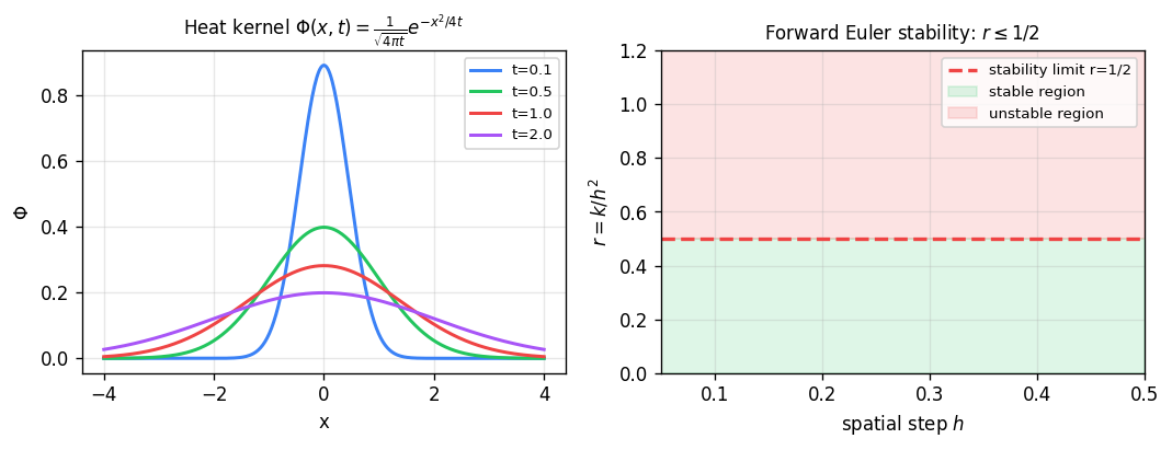
Left: the heat kernel \(\Phi(x,t) = \frac{1}{\sqrt{4\pi t}}e^{-x^2/4t}\) spreading and flattening as \(t\) grows. Right: stability constraint \(r = k/h^2 \le 1/2\) for the forward Euler (explicit) scheme — violating this bound causes exponential blow-up.

Inhomogeneous Heat Equation

For the problem \(u_t = \Delta u + f(x,t)\), \(u(x,0) = 0\) on \(\mathbb{R}^n\), the Duhamel principle and the convolution property of the Fourier transform \(\mathcal{F}\{f*g\} = \mathcal{F}\{f\}\mathcal{F}\{g\}\) yield the solution:

\[ u(x,t) = \int_0^t \int_{\mathbb{R}^n} K(x-y, t-s)\,f(y,s)\,dy\,ds. \]

The full solution to the IVP \(u_t = \Delta u + f\), \(u(x,0) = g(x)\) on \(\mathbb{R}^n\) is, by superposition:

\[ u(x,t) = \int_{\mathbb{R}^n} K^*(x-y,t)\,g(y)\,dy + \int_0^t\!\int_{\mathbb{R}^n} K^*(x-y,t-s)\,f(y,s)\,dy\,ds, \]

where \(K^*(x,t) = K(x,0,t) = (4\pi t)^{-n/2} e^{-|x|^2/(4t)}\) is the standard heat kernel.

Scaling Transformations

A powerful technique for reducing PDEs to ODEs is the similarity method. Consider the scaling \(\bar{u} = \varepsilon^\alpha u\), \(\bar{x} = \varepsilon^\beta x\), \(\bar{t} = \varepsilon^\gamma t\). If the PDE is invariant under this family of scalings for all \(\varepsilon > 0\), we can set \(\varepsilon^\gamma = t\) (i.e., normalize time to 1) and introduce the similarity variable \(z = t^{-\beta/\gamma} x\) and similarity solution \(w(z) = u(x,t)/t^{\alpha/\gamma}\), giving \(u(x,t) = t^{\alpha/\gamma} w(z)\).

For the heat equation \(u_t = \Delta u\), the scaling \(\alpha = 0\), \(\beta = -1\), \(\gamma = -2\) (or any scalar multiple) preserves the equation: \(\bar{u}_{\bar{t}} = \Delta_{\bar{x}}\bar{u}\). The similarity variable is \(z = x/\sqrt{t}\), and radial similarity solutions take the form \(w = w(|z|)\), satisfying the ODE

\[ w'' + \left(\frac{n-1}{r} + \frac{r}{2}\right)w' = 0, \quad r = |z|, \]

whose solution (with appropriate normalization) recovers the heat kernel \(K^*(x,t) = (4\pi t)^{-n/2}e^{-|x|^2/(4t)}\).