AMATH 353: Partial Differential Equations 1
E.R. Vrscay
Estimated study time: 2 hr 8 min
Table of contents
Chapter 1: Introduction to Partial Differential Equations
What is a PDE?
A partial differential equation (PDE) is an equation involving an unknown function \( u \) of two or more independent variables and certain of its partial derivatives. If \( u \) is a function of \( x \) and \( y \), then examples include:
\[ \frac{\partial u}{\partial x} + \frac{\partial u}{\partial y} = 0, \qquad u\frac{\partial^2 u}{\partial x^2} + \frac{\partial u}{\partial y} = 0, \qquad \frac{\partial^2 u}{\partial x^2} + \frac{\partial^2 u}{\partial y^2} = x^2 + y^2. \]Notice the contrast with an ordinary differential equation (ODE), which involves a function of a single variable and its ordinary derivatives. As soon as the unknown function depends on more than one variable, the equation necessarily becomes a PDE.
Much of this course is devoted to linear, second-order PDEs for two reasons: there is a reasonable mathematical theory for them, and they model an enormous variety of natural phenomena.
Why PDEs? The Transition from ODEs
ODEs are appropriate for modelling homogeneous or point-like systems: a mass on a spring, a projectile, a pendulum, or the temperature of a body small enough to be treated as having uniform temperature throughout. The moment spatial variation matters, PDEs become necessary.
Consider the temperature of a large steel ingot cooling in air. The surface cools first, and heat is conducted from the hot interior toward the surface. The temperature \( T \) is a function of both position and time: \( T = T(\mathbf{x}, t) \). Similarly, a chemical dissolving from a lump at the bottom of an unstirred beaker creates a concentration gradient \( c = c(\mathbf{x}, t) \). In both cases, the spatial dependence is the crucial new ingredient, and PDEs are the right tool.
In applications, the unknown function \( u \) typically depends on \( n \) spatial variables \( x_1, \ldots, x_n \) and one time variable \( t \):
\[ u = u(x_1, \ldots, x_n, t), \quad n = 1, 2, \text{ or } 3. \]The Three Canonical Types
The Heat (Diffusion) Equation
For a function \( u(x,t) \) depending on one spatial variable and time, the 1D heat equation is
\[ \frac{\partial u}{\partial t} = k \frac{\partial^2 u}{\partial x^2}. \]In higher dimensions, the single second derivative in \( x \) is replaced by the Laplacian \( \nabla^2 u \):
\[ \frac{\partial u}{\partial t} = k \nabla^2 u. \]In two and three dimensions respectively,
\[ \nabla^2 u = \frac{\partial^2 u}{\partial x^2} + \frac{\partial^2 u}{\partial y^2}, \qquad \nabla^2 u = \frac{\partial^2 u}{\partial x^2} + \frac{\partial^2 u}{\partial y^2} + \frac{\partial^2 u}{\partial z^2}. \]The heat equation is parabolic: it has one time derivative on the left and a second spatial derivative on the right.
The Wave Equation
The 1D wave equation is
\[ \frac{\partial^2 u}{\partial t^2} = c^2 \frac{\partial^2 u}{\partial x^2}, \]and in higher dimensions, \( \partial^2 u/\partial t^2 = c^2 \nabla^2 u \). This is a hyperbolic PDE, characterised by two time derivatives. The constant \( c \) is the wave speed.
Laplace’s Equation
If the heat equation is solved in the steady state (time-independent regime), then \( \partial u/\partial t = 0 \) and the equation reduces to Laplace’s equation:
\[ \nabla^2 u = 0. \]This is an elliptic PDE. Its solutions, called harmonic functions, describe equilibrium temperature distributions, electrostatic potentials, and irrotational fluid flow. When sources are present, the steady-state equation becomes Poisson’s equation:
\[ \nabla^2 u = f(\mathbf{x}). \]The Schrödinger Equation
An important linear PDE from quantum mechanics is the Schrödinger equation for a particle of mass \( m \) in a potential \( V(\mathbf{x}) \):
\[ i\hbar \frac{\partial u}{\partial t} = -\frac{\hbar^2}{2m} \nabla^2 u + V(\mathbf{x}) u, \]where \( \hbar = h/(2\pi) \) is the reduced Planck constant and \( u \) is the complex-valued wavefunction. This equation has the same structure as the heat equation (first-order in time, second-order in space), but with complex coefficients.
Initial and Boundary Conditions
A PDE alone does not determine a unique solution; additional data must be prescribed. The appropriate type of data depends on the type of equation.
- Initial conditions (for time-dependent problems): prescribe \( u(\mathbf{x}, 0) \), and for the wave equation, also \( u_t(\mathbf{x}, 0) \).
- Boundary conditions: specify the behaviour of \( u \) on the spatial domain boundary \( \partial \Omega \).
The three main types of boundary conditions are:
- Dirichlet: \( u = g \) on \( \partial \Omega \) (prescribed values).
- Neumann: \( \partial u / \partial n = h \) on \( \partial \Omega \) (prescribed normal derivative, hence flux).
- Robin (mixed): \( \alpha u + \beta \partial u/\partial n = g \) on \( \partial \Omega \).
The Modelling Framework: Conservation Laws
The conservation law derivation of the heat equation (given in full detail in Chapter 2) is a special case of a universal modelling template. Consider any extensive quantity \(u(x,t)\) — temperature, chemical concentration, traffic density, population — defined on a one-dimensional domain. The global conservation law for \(u\) over an arbitrary interval \([a,b]\) states:
\[ \frac{d}{dt}\int_a^b u\,dx = \phi(a,t) - \phi(b,t) + \int_a^b f\,dx, \]where \(\phi(x,t)\) is the flux (the rate at which \(u\) crosses the point \(x\) in the positive direction) and \(f(x,t)\) is the source density. Rewriting the flux terms as \(-\int_a^b \partial\phi/\partial x\,dx\) and invoking the Du Bois-Reymond lemma (since \([a,b]\) is arbitrary), one obtains the local conservation law:
\[ \frac{\partial u}{\partial t} + \frac{\partial \phi}{\partial x} = f. \]This is the universal skeleton of a PDE model. To close the system, one adds a constitutive relation specifying \(\phi\) and \(f\) in terms of \(u\). Different choices yield different PDEs:
| Constitutive relation | Source \(f\) | PDE | Name |
|---|---|---|---|
| \(\phi = -Du_x\) | \(0\) | \(u_t = Du_{xx}\) | Diffusion / Heat |
| \(\phi = cu\) | \(0\) | \(u_t + cu_x = 0\) | Advection |
| \(\phi = cu - Du_x\) | \(0\) | \(u_t + cu_x = Du_{xx}\) | Advection-Diffusion |
| \(\phi = -Du_x\) | \(ru(1-u/K)\) | \(u_t = Du_{xx} + ru(1-u/K)\) | Fisher-KPP |
| \(\phi = u^2/2\) | \(0\) | \(u_t + uu_x = 0\) | Inviscid Burgers |
| \(\phi = u^2/2 - \nu u_x\) | \(0\) | \(u_t + uu_x = \nu u_{xx}\) | Viscous Burgers |
The advection equation \(u_t + cu_x = 0\) is the simplest first-order PDE. Its general solution is \(u(x,t) = u(x-ct, 0)\): the initial profile is carried rigidly to the right at speed \(c\), without distortion. This will be confirmed via the method of characteristics in Chapter 12.
The Fisher-KPP equation (proposed independently by Fisher and by Kolmogorov, Petrovskii, and Piskunov in 1937) couples diffusion with logistic population growth. It supports travelling wave solutions — fronts that advance into unstratified territory at a minimum speed \(c^* = 2\sqrt{rD}\), determined by the interplay of diffusion and growth.
The Burgers equation \(u_t + uu_x = \nu u_{xx}\) combines nonlinear advection (with the solution value itself as advection speed) and linear diffusion. In the inviscid limit \(\nu \to 0\), profiles steepen and shocks form — the phenomena studied in Chapter 12. With viscosity, the Hopf-Cole transformation \(u = -2\nu(\ln v)_x\) converts it to the heat equation exactly, making Burgers the paradigm for exactly solvable nonlinear PDEs.
The recurring template — PDE = conservation law + constitutive relation — structures much of applied mathematics, from fluid dynamics and electromagnetism to population ecology. Every PDE studied in this course fits this mould.
Classification of Second-Order PDEs
A general second-order linear PDE in two independent variables \(x\) and \(y\) takes the form
\[ A u_{xx} + B u_{xy} + C u_{yy} + D u_x + E u_y + F u = G, \]where \(A, B, C, \ldots\) may depend on \(x\) and \(y\). The classification depends on the discriminant
\[ \Delta = B^2 - 4AC. \]- Hyperbolic if \(\Delta > 0\) — two real characteristic directions exist.
- Parabolic if \(\Delta = 0\) — one repeated characteristic direction.
- Elliptic if \(\Delta < 0\) — no real characteristics.
Verification for the canonical types. For the heat equation \(u_t = ku_{xx}\) (with variables \(x\) and \(t\)): \(A = k\), \(B = 0\), \(C = 0\), so \(\Delta = 0\) — parabolic. For the wave equation \(u_{tt} = c^2 u_{xx}\): \(A = -c^2\), \(B = 0\), \(C = 1\), giving \(\Delta = 4c^2 > 0\) — hyperbolic. For Laplace’s equation \(u_{xx} + u_{yy} = 0\): \(A = 1\), \(B = 0\), \(C = 1\), so \(\Delta = -4 < 0\) — elliptic.
Reduction to Canonical Form
The discriminant is not merely a label — it determines the geometry of characteristic curves, which are the curves along which information propagates. For a hyperbolic PDE, two families of characteristic curves satisfy
\[ \frac{dy}{dx} = \frac{B \pm \sqrt{B^2 - 4AC}}{2A}. \]Setting \(\xi = \xi(x,y)\) and \(\eta = \eta(x,y)\) as functions constant on each family, the transformed PDE takes the canonical hyperbolic form \(u_{\xi\eta} = \text{(lower-order terms)}\).
For the wave equation \(u_{tt} = c^2u_{xx}\), the characteristic curves satisfy \(dx/dt = \pm c\), giving the characteristic variables \(\xi = x - ct\) and \(\eta = x + ct\). In these coordinates, the wave equation reduces to
\[ \frac{\partial^2 u}{\partial \xi\,\partial \eta} = 0, \]which integrates immediately to \(u = F(\xi) + G(\eta) = F(x-ct) + G(x+ct)\) — d’Alembert’s solution.
Ill-Posedness and Hadamard’s Example
The classification has a decisive implication for well-posedness. For elliptic equations, specifying Cauchy data (both \(u\) and its normal derivative) on an open curve is a severely ill-posed problem. The classic counterexample due to Hadamard considers Laplace’s equation with oscillatory Neumann data:
\[ u_{xx} + u_{yy} = 0, \quad u(x,0) = 0, \quad u_y(x,0) = \frac{\sin(nx)}{n}. \]The exact solution is
\[ u_n(x,y) = \frac{\sin(nx)\sinh(ny)}{n^2}. \]As \(n \to \infty\), the Cauchy data \(u_y(x,0) = n^{-1}\sin(nx)\) tends to zero uniformly, yet for any fixed \(y > 0\),
\[ \|u_n(\cdot,y)\|_\infty = \frac{\sinh(ny)}{n^2} \sim \frac{e^{ny}}{2n^2} \to \infty. \]Vanishingly small changes in the data produce unbounded changes in the solution: this Cauchy problem for Laplace’s equation is not well-posed. The ill-posedness arises because the Laplacian has no preferred time direction — solutions can grow in either direction, and without a closed boundary to constrain them, arbitrarily small high-frequency perturbations explode. The same mechanism underlies the ill-posedness of the backward heat equation: running \(u_t = ku_{xx}\) in reverse (\(u_t = -ku_{xx}\)) causes high-wavenumber modes to grow as \(e^{+Dk^2|t|}\), amplifying any noise without bound.
Chapter 2: The Heat Equation in One Dimension
Physical Derivation
We model heat conduction in a uniform rod of length \( L \) and constant cross-sectional area \( A \). The rod lies along the \( x \)-axis, \( 0 \le x \le L \). We assume all heat flow is in the \( x \)-direction (the lateral surface is insulated).
Step 1: Thermal energy density. Define \( e(x,t) \) as the thermal energy per unit volume at position \( x \) and time \( t \). For a thin slice of width \( \Delta x \), the total thermal energy is \( \Delta h \approx e(x,t) A \Delta x \), and the total energy in the segment \( [a,b] \) is
\[ h(a,b;t) = \int_a^b e(x,t)\, A\, dx. \]Step 2: Conservation of energy. Changes in thermal energy in \( [a,b] \) are due only to heat flow across the boundaries and any internal sources:
\[ \frac{d}{dt} \int_a^b e(x,t)\, A\, dx = \phi(a,t) A - \phi(b,t) A + \int_a^b Q(x,t)\, A\, dx, \]where \( \phi(x,t) \) is the heat flux (thermal energy per unit time per unit area flowing in the positive \( x \)-direction), and \( Q(x,t) \) is the rate of thermal energy generated per unit volume. Applying the Fundamental Theorem of Calculus to the flux terms and combining:
\[ \int_a^b \left( \frac{\partial e}{\partial t} + \frac{\partial \phi}{\partial x} - Q \right) dx = 0. \]Since this holds for every interval \( [a,b] \) and the integrand is continuous, the Du Bois-Reymond lemma yields the differential form of conservation:
\[ \frac{\partial e}{\partial t} + \frac{\partial \phi}{\partial x} = Q. \]This lemma, which converts an integral law into a pointwise (differential) law, is used repeatedly throughout the course.
Step 3: Relating energy to temperature. Define the specific heat \( c(x) \) as the heat energy required to raise a unit mass by one unit of temperature, and let \( \rho(x) \) be the mass density. Then
\[ e(x,t) = c(x)\rho(x)\bigl[u(x,t) - u_0\bigr], \]where \( u(x,t) \) is the temperature and \( u_0 \) is a reference temperature (whose choice is irrelevant). Differentiating in time:
\[ c(x)\rho(x) \frac{\partial u}{\partial t} = -\frac{\partial \phi}{\partial x} + Q. \]Step 4: Fourier’s law. From experiment, heat flows from hotter regions to colder regions, at a rate proportional to the temperature gradient:
The minus sign ensures that heat flows in the direction of decreasing temperature. Substituting into the conservation equation gives the generalised heat equation:
\[ c(x)\rho(x) \frac{\partial u}{\partial t} = \frac{\partial}{\partial x}\!\left( K_0(x) \frac{\partial u}{\partial x} \right) + Q. \]For a homogeneous rod (constant \( c, \rho, K_0 \)) with no sources (\( Q = 0 \)), this simplifies to
\[ \frac{\partial u}{\partial t} = k \frac{\partial^2 u}{\partial x^2}, \]where the thermal diffusivity is \( k = K_0 / (c\rho) \). This is the 1D heat equation.
Separation of Variables: Dirichlet Boundary Conditions
We solve the 1D heat equation on \( [0,L] \) with zero-endpoint (Dirichlet) boundary conditions:
\[ \frac{\partial u}{\partial t} = k \frac{\partial^2 u}{\partial x^2}, \quad u(0,t) = 0, \quad u(L,t) = 0, \quad u(x,0) = f(x). \]We assume a solution of the form \( u(x,t) = \phi(x) G(t) \). Substituting:
\[ \phi(x) G'(t) = k \phi''(x) G(t) \implies \frac{G'(t)}{kG(t)} = \frac{\phi''(x)}{\phi(x)} = -\lambda, \]where \( \lambda \) is the separation constant. The two ODEs are:
\[ G'(t) + k\lambda G(t) = 0, \qquad \phi''(x) + \lambda \phi(x) = 0, \quad \phi(0) = \phi(L) = 0. \]Case \( \lambda < 0 \): The solution for \( \phi \) grows exponentially, violating the boundary conditions (only the trivial solution survives). Case \( \lambda = 0 \): Similarly, only the trivial solution exists. Case \( \lambda > 0 \): The general solution is \( \phi(x) = C_1 \cos(\sqrt{\lambda} x) + C_2 \sin(\sqrt{\lambda} x) \). The condition \( \phi(0) = 0 \) forces \( C_1 = 0 \). The condition \( \phi(L) = 0 \) then requires \( \sin(\sqrt{\lambda} L) = 0 \), so
\[ \sqrt{\lambda_n} L = n\pi \implies \lambda_n = \frac{n^2\pi^2}{L^2}, \quad n = 1, 2, 3, \ldots \]The eigenvalues are \( \lambda_n \) and the corresponding eigenfunctions are
\[ \phi_n(x) = \sin\!\left(\frac{n\pi x}{L}\right). \]These are the normal modes of the rod. The time-dependent part gives \( G_n(t) = e^{-k\lambda_n t} = e^{-k(n\pi/L)^2 t} \), so the separated solutions are
\[ u_n(x,t) = \sin\!\left(\frac{n\pi x}{L}\right) e^{-k(n\pi/L)^2 t}, \quad n = 1, 2, 3, \ldots \]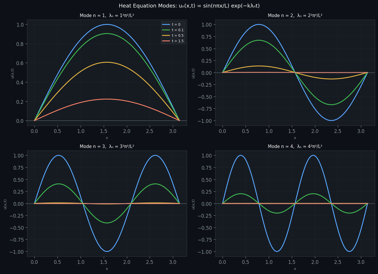
Fourier Sine Series
By the principle of superposition (valid for linear homogeneous equations), any linear combination of the \( u_n \) is also a solution. We seek coefficients \( c_n \) such that the initial condition is satisfied:
\[ u(x,0) = \sum_{n=1}^{\infty} c_n \sin\!\left(\frac{n\pi x}{L}\right) = f(x). \]The eigenfunctions are orthogonal on \( [0,L] \):
\[ \int_0^L \sin\!\left(\frac{m\pi x}{L}\right) \sin\!\left(\frac{n\pi x}{L}\right) dx = \begin{cases} 0, & m \ne n, \\ L/2, & m = n. \end{cases} \]Multiplying the expansion by \( \sin(m\pi x/L) \) and integrating gives the Fourier sine coefficients:
\[ c_n = \frac{2}{L} \int_0^L f(x) \sin\!\left(\frac{n\pi x}{L}\right) dx. \]The complete solution is
\[ u(x,t) = \sum_{n=1}^{\infty} c_n \sin\!\left(\frac{n\pi x}{L}\right) e^{-k(n\pi/L)^2 t}. \]Physical Interpretation of Each Mode
The \( n \)-th mode is a standing wave in space (with \( n \) half-periods fitting in \( [0,L] \)) multiplied by an exponentially decaying envelope in time. The first mode, \( n=1 \), is a single arch: the entire rod cools slowly. The \( n=2 \) mode has a node at \( x = L/2 \): the left half cools while the right half also cools, each independently. Higher modes represent finer spatial structures that decay more rapidly.
Superposition Principle
Chapter 3: Steady-State Solutions and Boundary Conditions
Equilibrium Temperature Distributions
A steady-state or equilibrium temperature distribution is one that is time-independent: \( u(x,t) = u_{eq}(x) \). Setting \( \partial u/\partial t = 0 \) in the 1D heat equation gives
\[ k \frac{d^2 u_{eq}}{dx^2} = 0 \implies \frac{d^2 u_{eq}}{dx^2} = 0 \implies u_{eq}(x) = C_1 x + C_2. \]The equilibrium solution is always linear in \( x \); the constants are determined by the boundary conditions.
For Dirichlet conditions \( u(0) = T_1 \), \( u(L) = T_2 \):
\[ u_{eq}(x) = T_1 + \frac{T_2 - T_1}{L} x. \]This is a linear interpolation between the two endpoint temperatures. We expect that all solutions to the heat equation with these boundary conditions will eventually approach this distribution.
Mixed Boundary Conditions
For a mixed problem, say \( u(0) = T_1 \) (fixed temperature at the left) and \( u'(L) = 0 \) (insulated right end), the equilibrium is
\[ u_{eq}(x) = T_1, \]a uniform constant temperature. Physically, the insulated right end cannot lose heat, so in steady state the rod equilibrates to the temperature imposed at the left.
Heat Sources
If a source term \( Q(x) \) is present, the equilibrium satisfies the ODE
\[ K_0 \frac{d^2 u_{eq}}{dx^2} = -Q(x), \]which may be integrated twice. The constants of integration are fixed by the boundary conditions.
The condition \( u(0) = 0 \) gives \( C_2 = 0 \). The condition \( u(1) = 0 \) gives \( C_1 = 1/6 \), so
\[ u_{eq}(x) = \frac{1}{6}(x - x^3) = \frac{x(1-x^2)}{6}. \]The flux at the endpoints is \( \phi(0) = -u'(0) = -1/6 \) and \( \phi(1) = -u'(1) = 1/3 \). The total rate of heat production is \( \int_0^1 x\, dx = 1/2 \). The net outward heat flow rate is \( \phi(1) - \phi(0) = 1/3 - (-1/6) = 1/2 \), confirming energy balance. \(\blacksquare\)
Non-existence of Steady State
If the rod is insulated at both ends (\( u'(0) = u'(L) = 0 \)) but has an internal source, energy accumulates indefinitely and no steady state exists. Mathematically, imposing \( u'(0) = 0 \) and \( u'(L) = 0 \) on the general solution \( u_{eq}' = -x^2/3 + C_1 \) forces \( C_1 = 0 \) and then \( L = 0 \), a contradiction. This confirms that heat production with no mechanism for escape precludes equilibrium.
Nonhomogeneous Boundary Conditions via Change of Variables
Separation of variables requires homogeneous boundary conditions. For nonhomogeneous conditions \( u(0) = A \) and \( u(L) = B \), we write \( u(x,t) = u_{eq}(x) + v(x,t) \), where \( u_{eq}(x) = A + (B-A)x/L \) is the unique steady state. Then \( v \) satisfies the homogeneous conditions \( v(0) = v(L) = 0 \) and the same heat equation. We then expand \( v \) in Fourier sine series as before.
Chapter 4: The Heat Equation — Neumann and Other Conditions
Zero-Flux (Neumann) Boundary Conditions
Neumann boundary conditions model an insulated rod: no heat flows in or out through the endpoints. The problem is
\[ \frac{\partial u}{\partial t} = k \frac{\partial^2 u}{\partial x^2}, \quad \frac{\partial u}{\partial x}(0,t) = 0, \quad \frac{\partial u}{\partial x}(L,t) = 0, \quad u(x,0) = f(x). \]Separation of variables with \( u = \phi(x) G(t) \) yields the same ODE for \( G(t) \), and the spatial problem
\[ \phi'' + \lambda \phi = 0, \quad \phi'(0) = 0, \quad \phi'(L) = 0. \]Applying the boundary conditions now gives the cosine eigenfunctions:
\[ \phi_n(x) = \cos\!\left(\frac{n\pi x}{L}\right), \quad \lambda_n = \frac{n^2\pi^2}{L^2}, \quad n = 0, 1, 2, \ldots \]Notice the crucial difference: the case \( n = 0 \) now produces the nontrivial eigenfunction \( \phi_0(x) = 1 \) (a constant) with eigenvalue \( \lambda_0 = 0 \). The time-dependent factor for \( n = 0 \) is \( G_0(t) = e^{0} = 1 \) — it does not decay. The general solution is
\[ u(x,t) = a_0 + \sum_{n=1}^{\infty} a_n \cos\!\left(\frac{n\pi x}{L}\right) e^{-k(n\pi/L)^2 t}. \]Cosine Series and Conservation
The initial condition \( u(x,0) = f(x) \) requires a Fourier cosine expansion:
\[ f(x) = a_0 + \sum_{n=1}^{\infty} a_n \cos\!\left(\frac{n\pi x}{L}\right), \]with coefficients
\[ a_0 = \frac{1}{L} \int_0^L f(x)\, dx, \qquad a_n = \frac{2}{L} \int_0^L f(x) \cos\!\left(\frac{n\pi x}{L}\right) dx, \quad n \ge 1. \]As \( t \to \infty \), all the oscillatory terms decay and
\[ u(x,t) \to a_0 = \frac{1}{L} \int_0^L f(x)\, dx. \]This is the spatial average of the initial temperature, which is precisely what conservation of thermal energy predicts: with insulated ends, the total thermal energy \( \int_0^L u(x,t)\, dx \) is constant in time (no heat escapes), so the final uniform temperature must equal the mean of the initial distribution.
Zero Eigenvalue and Non-uniqueness
The presence of \( \lambda_0 = 0 \) corresponds to the unique constant steady-state distribution \( u_{eq} = a_0 \). Unlike the Dirichlet problem (where \( u_{eq} = 0 \) is the only possibility), the Neumann problem admits a one-parameter family of steady states \( u_{eq} = C \) for any constant \( C \). The specific value to which the system evolves is determined solely by the initial data via conservation.
Chapter 5: The Heat Equation in Higher Dimensions
Multidimensional Conservation Law
The derivation of the heat equation in higher dimensions follows the same logic as in one dimension, using the Divergence Theorem in place of the Fundamental Theorem of Calculus. Let \( u(\mathbf{x}, t) \) be the temperature at position \( \mathbf{x} \in \mathbb{R}^n \) and time \( t \). Let \( D \subset \mathbb{R}^n \) be an arbitrary region bounded by a surface \( S \).
The heat flux vector \( \Phi(\mathbf{x}, t) \) is defined so that \( \Phi \cdot \hat{n}\, dS \) is the rate of outward heat flow through the surface element \( dS \) with outward unit normal \( \hat{n} \). Conservation of thermal energy states:
\[ \frac{d}{dt} \iiint_D e\, dV = -\iint_S \Phi \cdot \hat{n}\, dS + \iiint_D Q\, dV. \]Applying the Divergence Theorem to the surface integral, and using the Du Bois-Reymond lemma on the resulting combined integral over the arbitrary region \( D \):
\[ \frac{\partial e}{\partial t} = -\nabla \cdot \Phi + Q. \]The multidimensional version of Fourier’s law is
\[ \Phi = -K_0(\mathbf{x}) \nabla u, \]stating that heat flows in the direction of steepest temperature descent, at a rate proportional to the magnitude of the gradient. Substituting and using \( e = c\rho(u - u_0) \):
\[ c\rho \frac{\partial u}{\partial t} = \nabla \cdot (K_0 \nabla u) + Q. \]For a homogeneous medium with \( c, \rho, K_0 \) constant and no sources:
\[ \frac{\partial u}{\partial t} = k \nabla^2 u, \quad k = \frac{K_0}{c\rho}. \]The same argument for diffusion (using Fick’s law \( \phi = -k\nabla u \)) yields the identical equation for concentration \( u \). Incorporating chemical reactions leads to reaction-diffusion equations such as
\[ \frac{\partial u}{\partial t} = k \nabla^2 u - K u^2, \]which is nonlinear. This illustrates why the linearity of transport laws is so valuable.
2D Heat Equation on a Rectangle
On the rectangle \( 0 \le x \le L \), \( 0 \le y \le H \) with all edges held at zero temperature, separation of variables \( u = f(x)g(y)h(t) \) gives three ODEs. The result is a doubly-indexed family of normal modes:
\[ u_{mn}(x,y,t) = \sin\!\left(\frac{m\pi x}{L}\right) \sin\!\left(\frac{n\pi y}{H}\right) e^{-k\lambda_{mn} t}, \]where the 2D eigenvalues are
\[ \lambda_{mn} = \frac{m^2\pi^2}{L^2} + \frac{n^2\pi^2}{H^2}, \quad m, n = 1, 2, 3, \ldots \]The general solution is a double Fourier series:
\[ u(x,y,t) = \sum_{m=1}^{\infty} \sum_{n=1}^{\infty} B_{mn} \sin\!\left(\frac{m\pi x}{L}\right) \sin\!\left(\frac{n\pi y}{H}\right) e^{-k\lambda_{mn} t}. \]The coefficients \( B_{mn} \) are determined from the initial condition by double orthogonality.
Chapter 6: The Wave Equation
Vibrating String: Derivation
Consider a uniform elastic string of length \( L \) stretched under tension \( T_0 \) and displaced slightly from its equilibrium position. Let \( u(x,t) \) denote the transverse displacement. Applying Newton’s second law to a small element of the string of length \( \Delta x \) and mass \( \rho_0 \Delta x \) (where \( \rho_0 \) is the linear mass density), and assuming small displacements so that the horizontal component of tension is approximately constant, gives
\[ \rho_0 \frac{\partial^2 u}{\partial t^2} = T_0 \frac{\partial^2 u}{\partial x^2}, \]or, defining \( c^2 = T_0/\rho_0 \) (the square of the wave speed),
\[ \frac{\partial^2 u}{\partial t^2} = c^2 \frac{\partial^2 u}{\partial x^2}. \]This is the 1D wave equation. For a string clamped at both ends: \( u(0,t) = u(L,t) = 0 \). Initial conditions specify both the shape and velocity: \( u(x,0) = \alpha(x) \) and \( u_t(x,0) = \beta(x) \).
Normal Modes
Separating variables \( u(x,t) = \phi(x) h(t) \):
\[ \frac{h''(t)}{c^2 h(t)} = \frac{\phi''(x)}{\phi(x)} = -\lambda. \]The spatial problem is identical to the Dirichlet heat equation:
\[ \phi_n(x) = \sin\!\left(\frac{n\pi x}{L}\right), \quad \lambda_n = \frac{n^2\pi^2}{L^2}. \]The time equation \( h'' + c^2\lambda_n h = 0 \) has oscillatory solutions:
\[ h_n(t) = A_n \cos(\omega_n t) + B_n \sin(\omega_n t), \quad \omega_n = \frac{n\pi c}{L}. \]The natural frequencies are \( \omega_n = n\pi c / L \), \( n = 1, 2, 3, \ldots \). The fundamental frequency is \( \omega_1 = \pi c/L \), and higher modes are integer multiples thereof. This integer relationship — the harmonic series — is the mathematical basis of the musical overtones of a string instrument.
The general solution is:
\[ u(x,t) = \sum_{n=1}^{\infty} \sin\!\left(\frac{n\pi x}{L}\right) \left[ A_n \cos\!\left(\frac{n\pi c t}{L}\right) + B_n \sin\!\left(\frac{n\pi c t}{L}\right) \right], \]with \( A_n \) and \( B_n \) determined from the initial conditions by Fourier sine series.
d’Alembert’s Formula
The wave equation on the infinite line \( u_{tt} = c^2 u_{xx} \) admits a beautiful closed-form solution discovered by d’Alembert. Note that the PDE factors as
\[ \left(\frac{\partial}{\partial t} - c\frac{\partial}{\partial x}\right) \left(\frac{\partial}{\partial t} + c\frac{\partial}{\partial x}\right) u = 0. \]The general solution is a superposition of a right-travelling wave \( F(x - ct) \) and a left-travelling wave \( G(x+ct) \):
\[ u(x,t) = F(x - ct) + G(x + ct). \]Applying initial conditions \( u(x,0) = \alpha(x) \) and \( u_t(x,0) = \beta(x) \) gives d’Alembert’s formula:
\[ u(x,t) = \frac{\alpha(x-ct) + \alpha(x+ct)}{2} + \frac{1}{2c} \int_{x-ct}^{x+ct} \beta(s)\, ds. \]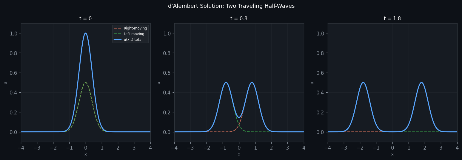
The quantities \( \xi = x - ct \) and \( \eta = x + ct \) are the characteristic variables: the solution is constant along each characteristic. The domain of dependence of the point \( (x_0, t_0) \) is the interval \( [x_0 - ct_0, x_0 + ct_0] \): the value of \( u \) at \( (x_0, t_0) \) is determined solely by the initial data in this interval.
2D Wave Equation: Vibrating Membrane
The equation \( u_{tt} = c^2 \nabla^2 u \) in two spatial dimensions models a thin elastic membrane. For a rectangular membrane \( [0,L] \times [0,H] \) clamped at all edges, separation of variables \( u = f(x)g(y)h(t) \) yields doubly-indexed normal modes with frequencies \( \omega_{mn} = c\sqrt{\lambda_{mn}} \), where \( \lambda_{mn} = (m\pi/L)^2 + (n\pi/H)^2 \). Unlike the string, these frequencies are generally not integer multiples of one another, which accounts for the inharmonic sound of drums.
Chapter 7: Laplace’s Equation and Harmonic Functions
Motivation
Laplace’s equation \( \nabla^2 u = 0 \) arises as the steady-state limit of the heat equation, as well as in electrostatics (electric potential \( V \) satisfies \( \nabla^2 V = -\rho/\varepsilon_0 \)), irrotational fluid flow, and gravitational potential theory. Solutions are called harmonic functions.
Rectangle: Separation of Variables
Consider \( \nabla^2 u = 0 \) on \( 0 \le x \le L \), \( 0 \le y \le H \) with prescribed boundary temperatures. With four nonhomogeneous conditions, the approach is to decompose \( u = u_1 + u_2 + u_3 + u_4 \), where each \( u_i \) satisfies one nonhomogeneous condition and three zero conditions.
For \( u_1 \), with \( u_1(x,0) = f_1(x) \) and the other three sides at zero, write \( u_1 = h(x)\phi(y) \). Separating:
\[ \frac{h''}{h} = -\frac{\phi''}{\phi} = -\lambda. \]The \( h \)-equation with zero boundary conditions at \( x = 0 \) and \( x = L \) gives \( h_n = \sin(n\pi x/L) \) and \( \lambda_n = (n\pi/L)^2 \). The \( \phi \)-equation is then \( \phi'' - (n\pi/L)^2 \phi = 0 \) with \( \phi(H) = 0 \). The solution convenient for imposing the boundary condition at \( y = H \) is
\[ \phi_n(y) = \sinh\!\left(\frac{n\pi}{L}(y - H)\right). \]The complete solution for \( u_1 \) is
\[ u_1(x,y) = \sum_{n=1}^{\infty} a_n \sin\!\left(\frac{n\pi x}{L}\right) \sinh\!\left(\frac{n\pi(y-H)}{L}\right), \]where the coefficients are
\[ a_n = \frac{-2}{L \sinh(n\pi H/L)} \int_0^L f_1(x) \sin\!\left(\frac{n\pi x}{L}\right) dx. \]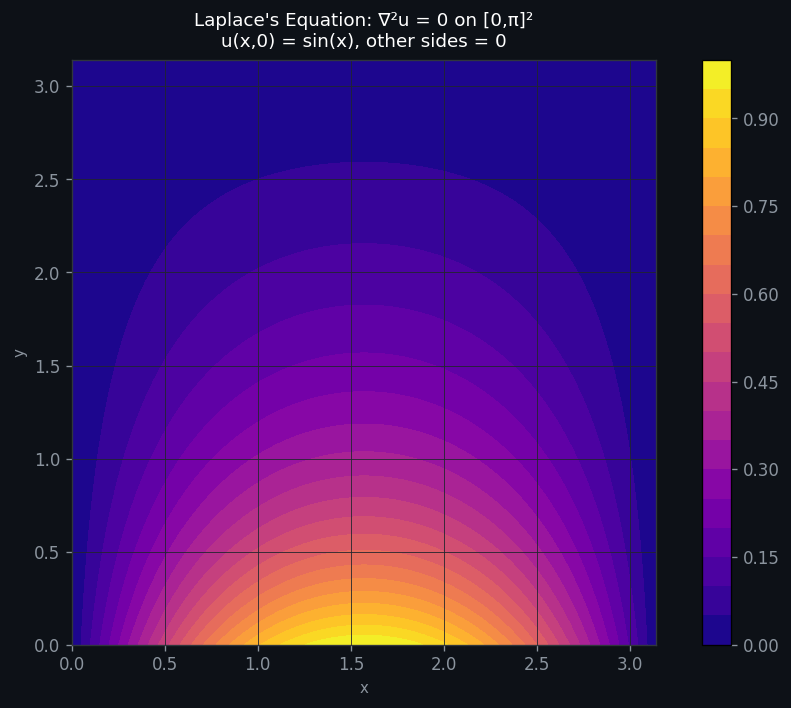
Laplace’s Equation on a Disk: Poisson Formula
For a circular disk of radius \( a \), it is natural to use polar coordinates \( (r,\theta) \). Laplace’s equation becomes
\[ \frac{1}{r}\frac{\partial}{\partial r}\!\left(r \frac{\partial u}{\partial r}\right) + \frac{1}{r^2}\frac{\partial^2 u}{\partial \theta^2} = 0. \]We seek \( u(r,\theta) \) satisfying the boundary condition \( u(a,\theta) = f(\theta) \) and the conditions of boundedness at \( r = 0 \) and periodicity in \( \theta \): \( u(r,-\pi) = u(r,\pi) \).
Setting \( u = G(r)\phi(\theta) \) and separating:
\[ \frac{r}{G}\frac{d}{dr}\!\left(r G'\right) = -\frac{\phi''}{\phi} = \mu_n = n^2, \quad n = 0, 1, 2, \ldots \]The periodicity condition on \( \phi \) forces \( \mu = n^2 \) for integer \( n \), with solutions \( \phi_n(\theta) = a_n \cos n\theta + b_n \sin n\theta \). The \( G \)-equation, a Cauchy-Euler equation, has solutions \( r^n \) and \( r^{-n} \). Boundedness at \( r = 0 \) excludes \( r^{-n} \) for \( n \ge 1 \). The general bounded solution is
\[ u(r,\theta) = a_0 + \sum_{n=1}^{\infty} r^n \bigl(a_n \cos n\theta + b_n \sin n\theta\bigr). \]Applying the boundary condition \( u(a,\theta) = f(\theta) \) and extracting the Fourier coefficients gives the Poisson integral formula (after summing the resulting geometric series):
\[ u(r,\theta) = \frac{a^2 - r^2}{2\pi} \int_{-\pi}^{\pi} \frac{f(\theta')}{a^2 - 2ar\cos(\theta - \theta') + r^2}\, d\theta'. \]The kernel \( P(r, \theta - \theta') = (a^2 - r^2) / (a^2 - 2ar\cos(\theta-\theta') + r^2) \) is called the Poisson kernel.
Chapter 8: Sturm-Liouville Theory and the Rayleigh Quotient
The General Sturm-Liouville Problem
The separation of variables procedure applied to PDEs with non-constant coefficients (e.g., a non-uniform rod with spatially varying \( K_0(x) \), \( c(x) \), \( \rho(x) \)) produces an ODE of the form
\[ \frac{d}{dx}\!\left(p(x) \frac{d\phi}{dx}\right) + q(x)\phi + \lambda \sigma(x) \phi = 0, \quad a < x < b, \]with homogeneous boundary conditions
\[ \beta_1 \phi(a) + \beta_2 \phi'(a) = 0, \qquad \beta_3 \phi(b) + \beta_4 \phi'(b) = 0. \]This is the regular Sturm-Liouville eigenvalue problem, provided \( p(x) > 0 \), \( \sigma(x) > 0 \), and \( p, q, \sigma \) satisfy appropriate smoothness conditions on \( [a,b] \). The standard Fourier problems (sine series, cosine series, full Fourier series) are all special cases corresponding to \( p = 1 \), \( q = 0 \), \( \sigma = 1 \).
- All eigenvalues \( \lambda_n \) are real.
- There are infinitely many eigenvalues: \( \lambda_1 < \lambda_2 < \cdots \), with \( \lambda_n \to \infty \).
- The eigenfunction \( \phi_n \) associated with \( \lambda_n \) has exactly \( n-1 \) zeros in \( (a,b) \).
- The eigenfunctions are orthogonal with weight \( \sigma(x) \): \[ \int_a^b \phi_m(x) \phi_n(x) \sigma(x)\, dx = 0 \quad \text{for } m \ne n. \]
- The eigenfunctions form a complete set (basis) for \( L^2_\sigma[a,b] \).
The orthogonality with weight \( \sigma \) arises because the Sturm-Liouville operator \( L = -\frac{d}{dx}(p\frac{d}{dx}) - q \) is self-adjoint with respect to the weighted inner product \( \langle f, g \rangle = \int_a^b fg\sigma\, dx \).
The Rayleigh Quotient
The Rayleigh quotient provides a variational characterisation of eigenvalues. For the simplified problem \( \phi'' + \lambda \sigma(x)\phi = 0 \), \( \phi(a) = \phi(b) = 0 \), one multiplies by \( \phi \) and integrates by parts to obtain
\[ \lambda = \frac{\int_a^b (\phi')^2\, dx}{\int_a^b \phi^2 \sigma(x)\, dx} = \text{RQ}(\phi). \]For the general Sturm-Liouville equation, the Rayleigh quotient is
\[ \text{RQ}(u) = \frac{-pu\,\frac{du}{dx}\Big|_a^b + \int_a^b \left[p(u')^2 - qu^2\right] dx}{\int_a^b u^2 \sigma\, dx}. \]- Trial function \( u_T = x(1-x) \): \( \text{RQ} = 10 \), relative error 1.3%.
- Hat function \( u_T \) (piecewise linear): \( \text{RQ} = 12 \), relative error 21%.
- Exact eigenfunction \( u_T = \sin\pi x \): \( \text{RQ} = \pi^2 \) exactly.
For the perturbed problem \( u'' + \lambda(1 + x/10)u = 0 \) on \( [0,\pi] \), the exact \( \lambda_1 \approx 0.8635 \), and the trial function \( \sin x \) gives \( \text{RQ} \approx 0.8642 \), an excellent approximation. \(\blacksquare\)
Connection to Quantum Mechanics
In quantum mechanics, the time-independent Schrödinger equation in one dimension is
\[ -\frac{\hbar^2}{2m} \psi''(x) + V(x)\psi(x) = E\psi(x), \]which is exactly a Sturm-Liouville eigenvalue problem with \( p = \hbar^2/(2m) \), \( q = -V(x) \), \( \sigma = 1 \), and eigenvalue \( E \) (the energy). The eigenfunctions \( \psi_n \) are the stationary states (orbitals) and the eigenvalues \( E_n \) are the allowed energy levels. The Rayleigh quotient in this context is the expectation value of the kinetic energy, providing a rigorous basis for the variational principle widely used in computational chemistry.
Chapter 9: The Circular Membrane and Bessel Functions
2D Wave Equation in Polar Coordinates
The vibration of a circular drum membrane of radius \( a \) is described by
\[ \frac{\partial^2 u}{\partial t^2} = c^2 \nabla^2 u = c^2\!\left(\frac{\partial^2 u}{\partial r^2} + \frac{1}{r}\frac{\partial u}{\partial r} + \frac{1}{r^2}\frac{\partial^2 u}{\partial \theta^2}\right), \]on \( 0 \le r \le a \), \( -\pi \le \theta \le \pi \), with boundary condition \( u(a,\theta,t) = 0 \) (clamped edge) and initial conditions on displacement and velocity.
Separation of Variables
We try \( u(r,\theta,t) = f(r)g(\theta)h(t) \). The time equation gives
\[ h''(t) + \lambda c^2 h(t) = 0 \implies h(t) = \cos(\sqrt{\lambda}\, ct) \text{ or } \sin(\sqrt{\lambda}\, ct), \]confirming oscillatory motion. The spatial factor satisfies \( \nabla^2\phi + \lambda\phi = 0 \) with \( \phi = f(r)g(\theta) \). Separating further:
\[ \frac{1}{\phi}\!\left(rf\right)'' / (rf) = -\frac{g''}{g} = m^2, \quad m = 0, 1, 2, \ldots \]The periodicity condition on \( g(\theta) \) forces \( m \) to be a non-negative integer, with
\[ g_m(\theta) = a_m \cos(m\theta) + b_m \sin(m\theta). \]The radial equation becomes
\[ r^2 f'' + r f' + (\lambda r^2 - m^2) f = 0, \]which, under the substitution \( s = \sqrt{\lambda}\, r \), transforms to Bessel’s equation of order \( m \):
\[ s^2 F'' + s F' + (s^2 - m^2) F = 0. \]Bessel Functions
The Bessel function \( Y_m(s) \) of the second kind is singular at \( s = 0 \); it is excluded by the boundedness condition \( |u(0,\theta,t)| < \infty \). Thus \( f_{mn}(r) = J_m(\sqrt{\lambda_{mn}}\, r) \).
The boundary condition \( u(a,\theta,t) = 0 \) requires \( J_m(\sqrt{\lambda_{mn}}\, a) = 0 \), so \( \sqrt{\lambda_{mn}}\, a = z_{mn} \), where \( z_{mn} \) is the \( n \)-th positive zero of \( J_m \). The eigenvalues are
\[ \lambda_{mn} = \left(\frac{z_{mn}}{a}\right)^2. \]The natural frequencies are \( \omega_{mn} = c\sqrt{\lambda_{mn}} = cz_{mn}/a \).
Normal Modes of the Circular Drum
The normal modes are
\[ u_{mn}(r,\theta,t) = J_m\!\left(\frac{z_{mn}}{a} r\right) (a_m \cos m\theta + b_m \sin m\theta) \cos(\omega_{mn} t). \]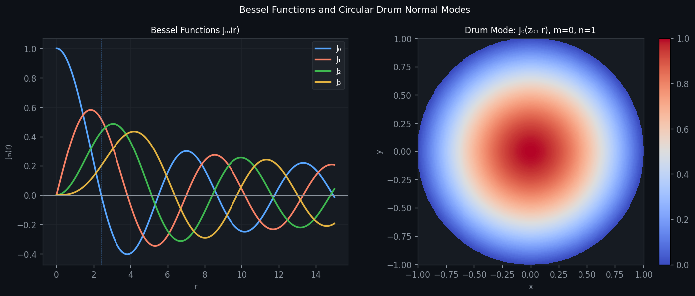
Radially symmetric modes (\( m = 0 \)): The mode \( u_{0n} = J_0(z_{0n} r/a) \cos(\omega_{0n} t) \). Since \( J_0 > 0 \) for \( 0 \le s < z_{0,1} \approx 2.405 \), the first mode (\( n=1 \)) has the entire membrane oscillating up and down uniformly — the two-dimensional analogue of the fundamental mode of a string. For \( n = 2 \), a nodal circle at radius \( r = (z_{0,1}/z_{0,2}) a \approx 0.44a \) divides the membrane into inner and outer regions oscillating out of phase.
Modes with angular dependence (\( m \ge 1 \)): The factor \( \cos(m\theta) \) introduces \( m \) nodal lines (diameters). For example, \( m = 1 \), \( n = 1 \) gives one nodal diameter, dividing the drum into two halves.
The weight \( r \) arises from the area element \( r\, dr\, d\theta \) in polar coordinates and is the manifestation of the Sturm-Liouville weight function \( \sigma = r \) in this context.
Chapter 10: Fourier Transforms and the Heat Equation on \( \mathbb{R} \)
From Fourier Series to Fourier Transforms
On a finite interval \( [-L, L] \), a function can be expanded in a Fourier series. As \( L \to \infty \), the discrete set of frequencies \( \omega_n = n\pi/L \) becomes a continuum, and the series becomes an integral. This limiting process motivates the Fourier transform.
and the inverse Fourier transform is
\[ f(x) = \mathcal{F}^{-1}\{F\}(x) = \int_{-\infty}^{\infty} F(\omega)\, e^{-i\omega x}\, d\omega. \]Key properties of the Fourier transform:
- Linearity: \( \mathcal{F}\{af + bg\} = a\mathcal{F}\{f\} + b\mathcal{F}\{g\} \).
- Derivative: \( \mathcal{F}\{\partial f/\partial x\} = -i\omega\, F(\omega) \), and iterating: \( \mathcal{F}\{\partial^2 f/\partial x^2\} = -\omega^2 F(\omega) \).
- Convolution: \( \mathcal{F}\{f * g\} = 2\pi\, \mathcal{F}\{f\} \cdot \mathcal{F}\{g\} \), where the convolution is \( (f*g)(x) = \int_{-\infty}^\infty f(x-s)g(s)\, ds \).
Solution of the Heat Equation on \( \mathbb{R} \)
The 1D heat equation on the whole real line with initial condition \( u(x,0) = f(x) \) is
\[ \frac{\partial u}{\partial t} = k\frac{\partial^2 u}{\partial x^2}, \quad x \in (-\infty,\infty), \quad u(x,t) \to 0 \text{ as } x \to \pm\infty. \]Taking the Fourier transform in \( x \) and using the derivative property:
\[ \frac{\partial U(\omega,t)}{\partial t} = -k\omega^2 U(\omega,t), \]where \( U(\omega,t) = \mathcal{F}\{u(\cdot,t)\}(\omega) \). This is a simple first-order ODE in \( t \) with solution
\[ U(\omega,t) = U(\omega,0)\, e^{-k\omega^2 t} = \mathcal{F}\{f\}(\omega)\, e^{-k\omega^2 t}. \]To invert, note that \( e^{-k\omega^2 t} \) is the Fourier transform (up to normalisation) of a Gaussian. Using the convolution theorem, the solution is
\[ u(x,t) = \int_{-\infty}^{\infty} f(s)\, h_t(x-s)\, ds = (f * h_t)(x), \]where the heat kernel (fundamental solution) is
\[ h_t(x) = \frac{1}{\sqrt{4\pi kt}}\, e^{-x^2/(4kt)}, \quad t > 0. \]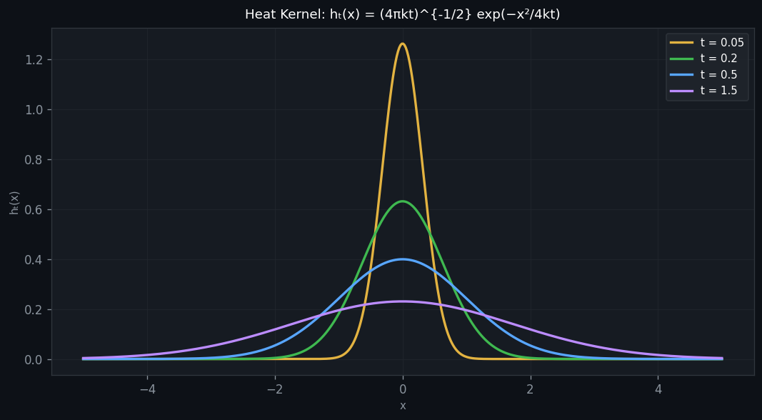
- \( h_t(x) > 0 \) for all \( x \in \mathbb{R} \) and \( t > 0 \): diffusion immediately spreads everywhere.
- \( \int_{-\infty}^\infty h_t(x)\, dx = 1 \) for all \( t > 0 \): total "probability" is conserved.
- As \( t \to 0^+ \), \( h_t(x) \to \delta(x) \): the Gaussian concentrates to a spike.
- The width of the Gaussian grows as \( \sqrt{4kt} \): the characteristic diffusion length scales as \( \sqrt{t} \).
Chapter 11: The Dirac Delta and Distributions
The Dirac Delta “Function”
The Dirac delta \( \delta(x) \) is not a function in the classical sense. It is defined by its action under integration: for any continuous \( f \),
\[ \int_{-\infty}^{\infty} f(x)\, \delta(x)\, dx = f(0), \qquad \int_{-\infty}^{\infty} f(x)\, \delta(x-x_0)\, dx = f(x_0). \]This sifting property expresses the fact that \( \delta(x - x_0) \) is a point mass concentrated at \( x_0 \). Informally, \( \delta(x) = 0 \) for \( x \ne 0 \) and \( \delta(0) = \infty \), with \( \int \delta(x)\, dx = 1 \).
The delta function is an example of a distribution (generalised function) — an object defined by its integration properties rather than pointwise values.
Fourier Transform of the Delta Function
Applying the definition of the Fourier transform directly:
\[ \mathcal{F}\{\delta(x)\}(\omega) = \frac{1}{2\pi} \int_{-\infty}^{\infty} \delta(x)\, e^{i\omega x}\, dx = \frac{1}{2\pi}. \]This is a remarkable result: a perfectly localised spike in space (\( \delta(x) \)) transforms to a perfectly uniform function in frequency space (\( 1/(2\pi) \)). Conversely, if \( F(\omega) = \delta(\omega) \), then
\[ f(x) = \int_{-\infty}^{\infty} \delta(\omega)\, e^{-i\omega x}\, d\omega = 1, \]a uniform function in space. This duality illustrates the Heisenberg uncertainty principle: a function that is perfectly concentrated in one domain is necessarily spread out in the other.
Integral Representation and Completeness
Substituting \( f(x) = \delta(x) \) and \( F(\omega) = 1/(2\pi) \) into the inverse Fourier transform formula yields the integral representation of the delta function:
\[ \delta(x) = \frac{1}{2\pi} \int_{-\infty}^{\infty} e^{-i\omega x}\, d\omega, \]or, with a shift,
\[ \delta(x - x_0) = \frac{1}{2\pi} \int_{-\infty}^{\infty} e^{-i\omega(x - x_0)}\, d\omega. \]This can be viewed as a completeness or resolution of the identity relation: expressing the kernel of the identity operator in terms of the plane wave basis \( \{e^{-i\omega x}\}_{\omega \in \mathbb{R}} \). The discrete analogue is
\[ \delta(x - x_0) = \sum_{n=1}^{\infty} \chi_n(x_0)\, \chi_n(x), \]where \( \{\chi_n\} \) is an orthonormal basis on an interval — this is the eigenfunction expansion of the delta function, fundamental to Green’s function theory.
Green’s Functions
The connection to PDEs: to solve \( Lu = f \) where \( L \) is a linear differential operator, one seeks the Green’s function \( G(x, x_0) \) satisfying \( LG = \delta(x - x_0) \) with appropriate boundary conditions. The solution is then
\[ u(x) = \int G(x, x_0)\, f(x_0)\, dx_0. \]The heat kernel \( h_t(x - s) \) is precisely the Green’s function of the heat operator \( \partial_t - k\partial_{xx} \) on the real line.
Two-Dimensional Fourier Transform
For \( f : \mathbb{R}^2 \to \mathbb{R} \), the 2D Fourier transform is
\[ F(\omega_1, \omega_2) = \frac{1}{(2\pi)^2} \iint_{\mathbb{R}^2} f(x_1,x_2)\, e^{i(\omega_1 x_1 + \omega_2 x_2)}\, dx_1\, dx_2 = \frac{1}{(2\pi)^2} \int_{\mathbb{R}^2} f(\mathbf{r})\, e^{i\boldsymbol{\omega}\cdot\mathbf{r}}\, d\mathbf{r}, \]with inverse \( f(\mathbf{x}) = \int_{\mathbb{R}^2} F(\boldsymbol{\omega})\, e^{-i\boldsymbol{\omega}\cdot\mathbf{x}}\, d\boldsymbol{\omega} \). The factored structure allows the 2D problem to be treated as two successive 1D transforms, one in each variable.
Chapter 12: Method of Characteristics
First-Order Linear PDEs
The method of characteristics reduces a first-order PDE to a system of ODEs. Consider the linear PDE
\[ \frac{\partial u}{\partial t} + c(x,t) \frac{\partial u}{\partial x} = Q(x,t,u). \]Along a curve \( x = x(t) \), the total derivative of \( u \) is
\[ \frac{du}{dt} = \frac{\partial u}{\partial t} + \frac{dx}{dt}\frac{\partial u}{\partial x}. \]If we choose the curve so that \( dx/dt = c \), then \( du/dt = Q \). The PDE reduces to the characteristic equations:
\[ \frac{dx}{dt} = c(x,t), \qquad \frac{du}{dt} = Q(x,t,u). \]The first equation defines the characteristic curves in the \( (x,t) \)-plane; along each characteristic, the second equation is an ODE for \( u \).
Quasilinear PDEs
For a quasilinear equation \( u_t + c(u,x,t)\, u_x = Q(u,x,t) \), the characteristics depend on the solution itself. The same procedure gives
\[ \frac{dx}{dt} = c(u,x,t), \qquad \frac{du}{dt} = Q(u,x,t). \]Traffic Flow
The method of characteristics finds its most vivid application in one-dimensional traffic flow. Let \( \rho(x,t) \) be the traffic density (cars per unit length) and \( q(x,t) \) the flux (cars per unit time). Conservation of cars on any interval \( [a,b] \) gives
\[ \frac{\partial \rho}{\partial t} + \frac{\partial q}{\partial x} = 0. \]Assuming the velocity \( u = u(\rho) \) is a decreasing function of density (dense traffic is slow), the flux is \( q = \rho u(\rho) = q(\rho) \). The conservation equation becomes
\[ \frac{\partial \rho}{\partial t} + q'(\rho)\frac{\partial \rho}{\partial x} = 0, \qquad c(\rho) = q'(\rho). \]This is a quasilinear PDE. The characteristic equations are \( d\rho/dt = 0 \) and \( dx/dt = c(\rho) \). Since \( \rho \) is constant along characteristics, \( c(\rho) \) is also constant, so the characteristics are straight lines:
\[ x(t) = c(\rho(x_0, 0))\, t + x_0. \]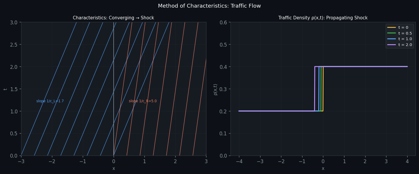
The Greenshields Model
A simple model for velocity: \( u(\rho) = u_{\max}(1 - \rho/\rho_{\max}) \), giving
\[ q(\rho) = u_{\max} \rho\!\left(1 - \frac{\rho}{\rho_{\max}}\right), \qquad c(\rho) = u_{\max}\!\left(1 - \frac{2\rho}{\rho_{\max}}\right). \]Note that \( c(\rho) \) can be negative for \( \rho > \rho_{\max}/2 \), corresponding to regions of very dense traffic where disturbances propagate backwards (upstream). This is the physical basis of traffic jams that move against the direction of travel.
Shock Waves and the Rankine-Hugoniot Condition
When initial data has a region where \( \rho(x_0, 0) > \rho(x_1, 0) \) for \( x_0 < x_1 \), the characteristics from \( x_0 \) and \( x_1 \) may converge and eventually intersect. At the intersection, \( \rho \) becomes multi-valued — the solution breaks down. This is the formation of a shock wave: a discontinuity in \( \rho \).
The physically correct way to handle shocks is to allow discontinuous solutions and enforce the Rankine-Hugoniot condition, which states that the speed \( V_s \) of the shock satisfies
\[ V_s = \frac{q(\rho_R) - q(\rho_L)}{\rho_R - \rho_L}, \]where \( \rho_L \) and \( \rho_R \) are the densities immediately to the left and right of the shock. This condition arises from demanding that the integral (weak) form of the conservation law hold across the discontinuity.
Chapter 13: Stability Theory and Dispersion
Normal Mode Analysis
Many PDEs of physical interest possess constant-coefficient solutions or equilibrium states whose stability one wants to assess: does a small perturbation decay, persist, or grow? The systematic tool is normal mode analysis, which exploits the translational symmetry of the coefficients to diagonalise the linearised problem.
Given a linear PDE with coefficients independent of \(x\) and \(t\), substitute the normal mode ansatz
\[ u(x,t) = e^{ikx + \lambda t} \]where \(k \in \mathbb{R}\) is the wavenumber and \(\lambda \in \mathbb{C}\) is the growth rate to be determined. Substituting into the PDE yields an algebraic equation relating \(\lambda\) to \(k\).
The diffusion equation \(u_t = Du_{xx}\): substituting gives \(\lambda = -Dk^2 \le 0\) for all \(k\). Every normal mode decays exponentially, with high-wavenumber (fine-scale) modes decaying fastest. The diffusion equation is unconditionally stable — it smooths initial data.
The backward heat equation \(u_t = -Du_{xx}\): now \(\lambda = +Dk^2 > 0\), and every mode grows, with short-wavelength perturbations growing fastest. This is the mechanism behind Hadamard’s ill-posedness result from Chapter 1: the backward problem is unstable in the most extreme sense.
Reaction-diffusion \(u_t = Du_{xx} + \alpha u\) (with \(\alpha > 0\)): the growth rate is \(\lambda = -Dk^2 + \alpha\). Long-wavelength modes (\(k^2 < \alpha/D\)) have \(\lambda > 0\) and grow, while short-wavelength modes are damped by diffusion. This competition between short-scale stabilisation and long-scale instability is the mathematical basis of Turing instability — the mechanism by which reaction-diffusion systems can spontaneously form spatial patterns from a uniform state.
The normal mode analysis for the heat equation reveals a quantitative version of the smoothing property: the solution operator \(e^{tL}\) is a low-pass filter in Fourier space, multiplying the \(k\)-th Fourier coefficient by \(e^{-Dk^2t}\). This is exactly the convolution with the heat kernel seen in Chapter 10.
Dispersion Relations
For wave-like problems, it is natural to recast the normal mode in terms of an explicitly oscillatory form. The travelling wave ansatz
\[ u(x,t) = e^{i(kx - \omega t)} \]is related to the normal mode by \(\lambda = -i\omega\). The relationship \(\omega = \omega(k)\) — the dispersion relation — encodes all the wave-propagation properties of the PDE. The phase speed
\[ c_p = \frac{\omega}{k} \]is the velocity at which crests of constant phase travel. A PDE is non-dispersive if \(c_p\) is independent of \(k\) (all wavenumbers travel at the same speed), and dispersive otherwise.
The wave equation \(u_{tt} = c^2 u_{xx}\): substituting gives \(-\omega^2 = -c^2k^2\), so \(\omega = \pm ck\) and \(c_p = \pm c\). The wave equation is non-dispersive: initial profiles propagate without change of shape — an initial Gaussian emerges as a perfect Gaussian at any later time.
The telegrapher’s equation \(u_{tt} + 2\gamma u_t = c^2 u_{xx}\) arises in transmission line theory, modelling electromagnetic waves with resistive losses. Substituting the travelling wave ansatz:
\[ -\omega^2 - 2i\gamma\omega = -c^2k^2 \implies \omega = -i\gamma \pm \sqrt{c^2k^2 - \gamma^2}. \]The imaginary part \(-\gamma\) of \(\omega\) causes uniform exponential damping (\(e^{-\gamma t}\)); the real part gives oscillation with phase speed
\[ c_p = \frac{\sqrt{c^2k^2 - \gamma^2}}{k} = c\sqrt{1 - \frac{\gamma^2}{c^2k^2}}, \]which approaches \(c\) as \(k \to \infty\) — low-frequency waves are slower, making the telegrapher’s equation dispersive and dissipative.
The Klein-Gordon equation \(u_{tt} = c^2 u_{xx} - \alpha^2 u\) (with \(\alpha > 0\)) arises in relativistic quantum mechanics and field theory as the wave equation for massive particles. The dispersion relation is
\[ \omega = \pm\sqrt{c^2k^2 + \alpha^2}, \]giving phase speed \(c_p = \pm\sqrt{c^2 + \alpha^2/k^2}\). Remarkably, \(c_p > c\) for all finite \(k\) — the phase velocity is superluminal! However, the group velocity
\[ c_g = \frac{d\omega}{dk} = \frac{c^2 k}{\sqrt{c^2k^2 + \alpha^2}} = \frac{c^2}{c_p} < c \]is subluminal. Since \(c_g\) is the velocity of energy and information propagation, special relativity is not violated.
The distinction between phase and group velocity is fundamental. A wave packet built from wavenumbers near \(k_0\) travels at the group velocity \(c_g(k_0)\), while the individual crests inside the packet move at the phase velocity \(c_p(k_0)\). For a non-dispersive medium, \(c_g = c_p\) and the packet maintains its shape; for a dispersive medium, the packet spreads over time as its constituent frequencies separate. This spreading is why, for example, a lightning strike (a broadband impulsive source) is heard as a rumble rather than a sharp crack at large distances — the atmosphere is dispersive.
Chapter 14: Adjoint Operators and Green’s Identities
The Adjoint of a Differential Operator
The concept of the adjoint of a linear operator is a far-reaching generalisation of the matrix transpose. For a differential operator \(L\) acting on functions on a domain \(\Omega\), the adjoint \(L^*\) is defined by the identity
\[ \langle v, Lu \rangle = \langle L^*v, u \rangle \]for all functions \(u, v\) in the function space, where \(\langle f, g \rangle = \int_\Omega fg\,d\mathbf{x}\) is the \(L^2\) inner product. Equivalently, \(L^*\) is the operator making the Green’s identity
\[ \int_\Omega \bigl(v\, Lu - u\, L^*v\bigr)\,d\mathbf{x} = \text{boundary terms} \]hold. The boundary terms are determined by integration by parts and depend on the domain and the boundary conditions imposed. If \(L^* = L\), the operator is self-adjoint — the PDE analogue of a symmetric matrix.
The Heat Operator and Its Adjoint
The heat operator \(L = \partial_t - k\partial_{xx}\) acts on functions of \((x,t)\). To find \(L^*\), multiply \(Lu\) by a test function \(v\) and integrate by parts over the space-time rectangle \([0,\ell] \times [0,T]\):
\[ \int_0^T\!\int_0^\ell v\,(u_t - ku_{xx})\,dx\,dt = \int_0^T\!\int_0^\ell u\,(-v_t - kv_{xx})\,dx\,dt + \text{(boundary terms)}. \]The time integration by parts gives \(\int v u_t\,dt = [vu]_0^T - \int u v_t\,dt\); the spatial integration by parts gives \(\int v u_{xx}\,dx = [vu_x - v_x u]_0^\ell + \int u v_{xx}\,dx\). Reading off the operator acting on \(u\) in the bulk integral, the adjoint is
\[ L^* v = -v_t - kv_{xx}. \]The heat operator is not self-adjoint: \(L^* \ne L\) because \(-\partial_t \ne \partial_t\). Physically, this reflects the irreversibility of diffusion — the forward and backward heat equations are genuinely different physical processes. The adjoint \(L^*\) corresponds to running the heat equation backward in time.
Self-Adjointness of the Laplacian
The Laplacian \(-\nabla^2\) (and more generally, any Sturm-Liouville operator \(L = -(pu')' + qu\) with appropriate boundary conditions) is self-adjoint. Green’s second identity states that for any smooth \(u, v\) on a domain \(\Omega\):
\[ \int_\Omega \bigl(v\nabla^2 u - u\nabla^2 v\bigr)\,d\mathbf{x} = \oint_{\partial\Omega}\bigl(v\nabla u - u\nabla v\bigr)\cdot\hat{n}\,dS. \]When \(u\) and \(v\) both satisfy homogeneous Dirichlet or Neumann boundary conditions on \(\partial\Omega\), the right-hand side vanishes, giving \(\langle v, Lu \rangle = \langle u, Lv \rangle\) — self-adjointness. This single identity is the engine behind all the orthogonality results of the course: the orthogonality of Fourier modes, of Bessel functions, and of Sturm-Liouville eigenfunctions all follow from Green’s second identity applied to eigenfunctions with different eigenvalues.
In Chapter 8, the Sturm-Liouville problem was treated as a boundary-value problem with a weight function. The abstract reason why distinct eigenfunctions are orthogonal is now clear: if \(L\phi_m = \lambda_m \sigma \phi_m\) and \(L\phi_n = \lambda_n \sigma \phi_n\), then self-adjointness (with the weight \(\sigma\)) gives
\[ (\lambda_m - \lambda_n)\langle \phi_m, \phi_n \rangle_\sigma = 0, \]so \(\langle \phi_m, \phi_n \rangle_\sigma = 0\) whenever \(\lambda_m \ne \lambda_n\).
Solvability and the Fredholm Alternative
The adjoint governs not just eigenvalue theory but the solvability of inhomogeneous equations. The central result is:
In words: the right-hand side \(f\) must be orthogonal to all solutions of the homogeneous adjoint problem. This is the PDE analogue of the familiar linear algebra result: the system \(A\mathbf{x} = \mathbf{b}\) has a solution if and only if \(\mathbf{b}\) is orthogonal to the null space of \(A^T\). The Fredholm alternative controls when Green’s functions exist and when resonance phenomena occur (the forcing \(f\) excites a natural mode of the system, leading to the absence of bounded solutions).
Chapter 15: Nonlinear Wave Phenomena and the KdV Equation
Linear Dissipation versus Linear Dispersion
The linear wave equation \(u_{tt} = c^2 u_{xx}\) propagates all Fourier modes at the same speed \(c\) with no change in amplitude. Two physically important modifications break this ideal behaviour:
Linear dissipation arises from resistive forces. For the advection-diffusion equation \(u_t + cu_x = \nu u_{xx}\), substituting \(u = e^{i(kx-\omega t)}\) gives
\[ -i\omega + ick = \nu(ik)^2 = -\nu k^2 \implies \omega = ck - i\nu k^2. \]The complex phase speed is \(U = \omega/k = c - i\nu k\), with a negative imaginary part proportional to \(k\). All modes are damped by the factor \(e^{-\nu k^2 t}\); short wavelengths (\(|k|\) large) decay fastest. This is dissipative but not dispersive: \(\mathrm{Re}(\omega)/k = c\) is independent of \(k\), so undamped components all travel at the same speed.
Linear dispersion arises from higher-order spatial derivatives. For \(u_t + cu_x + \beta u_{xxx} = 0\), substituting gives
\[ -i\omega + ick + \beta(ik)^3 = 0 \implies \omega = ck - \beta k^3, \quad U = c - \beta k^2. \]There is no damping (\(\mathrm{Im}(\omega) = 0\)), but the phase speed \(U = c - \beta k^2\) depends on \(k\): short waves travel at a different speed than long waves. A localised initial profile will spread as its Fourier components separate — dispersing without dissipating.
The Korteweg-de Vries Equation
In 1895, Korteweg and de Vries derived a model for long shallow-water waves that combines nonlinear steepening (like Burgers’ equation) with linear dispersion (the \(u_{xxx}\) term):
\[ u_t + 6uu_x + u_{xxx} = 0. \]This is the Korteweg-de Vries (KdV) equation. The nonlinear term \(6uu_x\) tends to steepen wave fronts — taller parts of the wave travel faster, causing the profile to lean forward and eventually break, as in Burgers’ equation. The dispersive term \(u_{xxx}\) opposes this: it spreads energy across wavenumbers, preventing blow-up. For a precise balance between the two effects, stable localised solutions exist.
The motivation for the KdV equation was the solitary wave observed by John Scott Russell on the Union Canal near Edinburgh in 1834. Russell followed a hump of water on horseback for two miles, noting that it maintained its shape and speed rather than spreading out or breaking. The existence of such waves was theoretically controversial for decades; KdV resolved the puzzle by providing an equation for which exact localised solutions exist.
The Soliton Solution
We seek a travelling wave \(u(x,t) = f(\xi)\) with \(\xi = x - Ut\) and wave speed \(U > 0\). Substituting into KdV:
\[ -Uf' + 6ff' + f''' = 0. \]Integrating once with respect to \(\xi\):
\[ f'' = Uf - 3f^2 + A \]for an integration constant \(A\). For a soliton — a localised pulse with \(f, f', f'' \to 0\) as \(|\xi| \to \infty\) — we need \(A = 0\). Multiplying by \(f'\) and integrating again:
\[ \frac{(f')^2}{2} = \frac{Uf^2}{2} - f^3 + B, \]and the same boundary condition forces \(B = 0\), giving
\[ (f')^2 = Uf^2 - 2f^3 = f^2(U - 2f). \]For a positive, localised solution, we need \(0 < f < U/2\). Taking the square root and separating variables, the integral can be evaluated by the substitution \(f = (U/2)\mathrm{sech}^2(\theta)\). One verifies directly (using \((\mathrm{sech}^2)'' = 2\mathrm{sech}^2(2\mathrm{sech}^2 - 1)\)) that the solution is
\[ f(\xi) = \frac{U}{2}\,\mathrm{sech}^2\!\left(\frac{\sqrt{U}}{2}\,\xi\right). \]Several features of this solution are extraordinary:
- Amplitude determines speed: there is no free parameter separating the height and velocity of a KdV soliton. A taller soliton is necessarily faster.
- Elastic collisions: when two KdV solitons collide, they pass through each other and emerge with their shapes and speeds completely unchanged — only a phase shift marks the interaction. This particle-like behaviour gave solitons their name.
- Stability: solitons are stable to small perturbations. This is the mathematical explanation for Russell’s observation: a solitary wave on a canal maintains its shape because the KdV balance between steepening and dispersion is dynamically stable.
The Inverse Scattering Transform
The KdV equation is a member of a rare class of completely integrable PDEs that can be solved exactly for arbitrary initial data. The inverse scattering transform (developed by Gardner, Greene, Kruskal, and Miura in 1967) proceeds in three steps:
- Direct scattering: the initial condition \(u(x,0)\) is treated as a potential in a Schrödinger equation \(\psi_{xx} + (\lambda - u)\psi = 0\); the bound-state eigenvalues \(\lambda_n < 0\) are computed.
- Time evolution: the scattering data evolve trivially in time — each eigenvalue is conserved, and the corresponding eigenfunction evolves as \(e^{4\lambda_n^{3/2}t}\).
- Inverse scattering: the solution \(u(x,t)\) is recovered from the evolved scattering data via the Gel’fand-Levitan-Marchenko integral equation.
Each bound state eigenvalue corresponds to a soliton in the long-time solution; the number of solitons is determined by the initial data. Continuous spectrum components disperse to zero, leaving a finite train of solitons as the asymptotic state. The inverse scattering transform is a nonlinear analogue of the Fourier transform: just as the Fourier transform linearises convolution, the IST linearises the KdV flow on the space of potentials.
The discovery of the IST opened the field of integrable systems, connecting KdV to the nonlinear Schrödinger equation, the sine-Gordon equation, and dozens of other exactly solvable models — one of the deepest developments in twentieth-century mathematical physics.
Appendix: Electrostatics and the Divergence Theorem
The material in the appendix (Set 2) establishes the Gauss Divergence Theorem and uses it to prove Gauss’ Law in electrostatics — an important model for how flux integrals underlie PDEs.
Gauss’ Law from the Divergence Theorem
For a point charge \( Q \) at the origin, the electrostatic field is
\[ \mathbf{E}(\mathbf{r}) = \frac{Q}{4\pi\varepsilon_0} \frac{\mathbf{r}}{r^3}. \]It can be shown that \( \nabla \cdot \mathbf{E} = 0 \) everywhere except at the origin. For a sphere \( S_R \) of radius \( R \), the outward flux is
\[ \iint_{S_R} \mathbf{E} \cdot \hat{n}\, dS = \frac{Q}{\varepsilon_0}, \]independent of \( R \). For an arbitrary surface \( S \) enclosing \( Q \), we introduce a small sphere \( S_\epsilon \) around the charge, apply the Divergence Theorem to the region between the two surfaces (where \( \nabla \cdot \mathbf{E} = 0 \)), and conclude that the flux through \( S \) equals \( Q/\varepsilon_0 \). This is Gauss’ Law.
In differential form, for a continuous charge distribution \( \rho(\mathbf{r}) \):
\[ \nabla \cdot \mathbf{E} = \frac{\rho}{\varepsilon_0}. \]Writing \( \mathbf{E} = -\nabla V \) yields Poisson’s equation for the electrostatic potential:
\[ \nabla^2 V = -\frac{\rho}{\varepsilon_0}. \]This is a fundamental PDE of physics, derivable from Gauss’ Law and the Divergence Theorem — the same combination of physical conservation and mathematical machinery that underlies all PDEs studied in this course. The recurring theme: PDE = conservation law + constitutive relation.
Summary and Connections
The Three Canonical PDEs: A Unified View
The three canonical second-order linear PDEs — heat, wave, and Laplace — share a common origin in conservation laws but differ in their time structure:
| PDE | Type | Time | Character |
|---|---|---|---|
| \( u_t = k\nabla^2 u \) | Parabolic | First order | Irreversible diffusion |
| \( u_{tt} = c^2\nabla^2 u \) | Hyperbolic | Second order | Reversible propagation |
| \( \nabla^2 u = 0 \) | Elliptic | None | Equilibrium |
Each was derived from a conservation law (of thermal energy, of momentum, or as a steady state) combined with a constitutive relation (Fourier’s law, Newton’s second law, or no-source condition). This structure — conservation + constitutive relation — is the template for PDE modelling throughout applied mathematics.
Fourier’s Vision
Joseph Fourier’s 1822 treatise Théorie analytique de la chaleur introduced the heat equation and the technique of expanding solutions in trigonometric series. The key insight — now called the completeness of the trigonometric system — is that virtually any function can be represented as an infinite sum of sines and cosines. This is the foundation of:
- The solution by Fourier sine/cosine series for the heat equation on \( [0,L] \).
- The Poisson integral formula for Laplace’s equation on a disk.
- The normal mode decomposition of the wave equation.
- The Fourier transform and the heat kernel on \( \mathbb{R} \).
Eigenvalues and Physical Quantisation
The discretisation of the separation constant — the appearance of a countable set of eigenvalues \( \lambda_1 < \lambda_2 < \cdots \) — is a mathematical reflection of a physical fact: bounded domains select preferred frequencies. This appears in:
- The natural frequencies \( \omega_n = n\pi c/L \) of a vibrating string.
- The energy levels \( E_n \propto n^2 \) of a particle in a box (quantum mechanics).
- The zeros \( z_{mn} \) of Bessel functions determining the drum’s frequencies.
All of these are manifestations of the Sturm-Liouville theory developed in Chapter 8. The elegant mathematics — self-adjoint operators, orthogonal eigenfunctions, complete bases — underlies both classical and quantum mechanics.
From Finite to Infinite: The Fourier Transform
The passage from Fourier series (finite interval) to Fourier transforms (whole real line) replaces a discrete sum over integers by a continuous integral over frequencies. The key parallel:
- Orthogonal eigenfunctions \( \phi_n(x) = \sin(n\pi x/L) \) become plane waves \( e^{-i\omega x} \).
- Coefficients \( c_n \) become the transform function \( F(\omega) \).
- Completeness (Parseval’s theorem) in the discrete case becomes the Plancherel theorem in the continuous case.
- The Dirac delta \( \delta(x-x_0) \) is the continuous analogue of the Kronecker delta, expressing the completeness of the plane wave basis.
Nonlinearity and Shocks
The course ends with first-order quasilinear PDEs and the method of characteristics, introducing the qualitatively new phenomenon of shock waves. The linearity enjoyed throughout Chapters 2–11 fails dramatically: nonlinear equations can develop singularities (shocks) in finite time from smooth initial data. The Rankine-Hugoniot condition, derived from the integral form of the conservation law, provides the unique physically consistent shock speed. Traffic flow is a prototype, but the same mathematics governs gas dynamics, water waves, and many other physical systems.
Remarks on Well-Posedness
Well-posedness (existence, uniqueness, continuous dependence on data) was verified in each chapter:
- For the heat equation with Dirichlet BCs: the Fourier sine series converges and provides a unique smooth solution; small changes in \( f(x) \) produce small changes in \( u(x,t) \).
- For the wave equation: the d’Alembert formula gives explicit existence and uniqueness; stability follows from the energy estimate.
- For Laplace’s equation: uniqueness follows from the maximum principle; existence requires more work (generally an integral equation).
- For the heat equation on \( \mathbb{R} \): the convolution formula \( u = f * h_t \) is explicit; \( h_t \in L^1(\mathbb{R}) \) with \( \|h_t\|_1 = 1 \) gives \( \|u(\cdot,t)\|_\infty \le \|f\|_\infty \).
This consistency between physical intuition and mathematical structure — instability in the heat equation run backward in time, the finite speed of wave propagation, the smoothing property of diffusion — is part of what makes PDEs such a powerful and intellectually satisfying subject.
